mjbroerman / bullseye

Locate points in polygons

bullseye 🎯

The goal of bullseye is to make it easy to build and serve point-in-polygon queries quickly. Under the hood, it uses the great new packages geoarrow and rsgeo.

Installation

You can install the development version of bullseye like so:

remotes::install_github("mjbroerman/bullseye)

Example

Given an address, the US Census free API service will assign coordinates and FIPS code to it. tidygeocoder will help.

In medical research, however, sharing personal identifying information (PII) with third-parties is not allowed. Nominatim, powered by OpenStreetMap will assign coordinates for you. For the FIPS codes, bullseye will help.

Currently bullseye can only build from census resources. The plan is to expand this arbitrary directories containing geometries.

Here we retrieve Alabama census block groups.

library(bullseye)
library(geoarrow)
library(dplyr)
#> 
#> Attaching package: 'dplyr'
#> The following objects are masked from 'package:stats':
#> 
#>     filter, lag
#> The following objects are masked from 'package:base':
#> 
#>     intersect, setdiff, setequal, union


# create db
poly_db_name <- "test_cen.parquet"
main_pipeline(base_url = "https://www2.census.gov/geo/tiger/TIGER2021/BG/",
              filename = poly_db_name,  
              n_limit = 2,
              save = FALSE) # default is TRUE, but vignettes disallow saving.
#> Reading layer `tl_2021_01_bg' from data source 
#>   `/private/var/folders/bp/l5qt50g13sndlz0x48jqqv300000gn/T/Rtmp3mAhLl/tl_2021_01_bg/tl_2021_01_bg.shp' 
#>   using driver `ESRI Shapefile'
#> Simple feature collection with 3925 features and 12 fields
#> Geometry type: MULTIPOLYGON
#> Dimension:     XY
#> Bounding box:  xmin: -88.47323 ymin: 30.14442 xmax: -84.88825 ymax: 35.00803
#> Geodetic CRS:  NAD83
#> Reading layer `tl_2021_02_bg' from data source 
#>   `/private/var/folders/bp/l5qt50g13sndlz0x48jqqv300000gn/T/Rtmp3mAhLl/tl_2021_02_bg/tl_2021_02_bg.shp' 
#>   using driver `ESRI Shapefile'
#> Simple feature collection with 504 features and 12 fields
#> Geometry type: MULTIPOLYGON
#> Dimension:     XY
#> Bounding box:  xmin: -179.2311 ymin: 51.17509 xmax: 179.8597 ymax: 71.43979
#> Geodetic CRS:  NAD83

Once built, we can query.

# simulate points
data("al_coord")
al_coord |> head()
#> Simple feature collection with 6 features and 1 field
#> Geometry type: POINT
#> Dimension:     XY
#> Bounding box:  xmin: -87.92333 ymin: 30.41867 xmax: -85.42765 ymax: 34.71424
#> Geodetic CRS:  WGS 84
#>                     geometry STATEFP
#> 1 POINT (-87.51496 31.58037)      01
#> 2 POINT (-86.36208 33.98386)      01
#> 3 POINT (-87.92333 32.16309)      01
#> 4 POINT (-85.42765 34.43848)      01
#> 5 POINT (-85.44814 34.71424)      01
#> 6 POINT (-86.77961 30.41867)      01

# load db
filepath <- system.file("extdata", poly_db_name, package = "bullseye")
test_db <- geoarrow::read_geoparquet_sf(filepath)

# query db
res <- combined_spatial_join(pts_sf = al_coord,
                      polys_sf = test_db,
                      prefilter_col = "STATEFP", 
                      return_col = "GEOID")

res
#> Simple feature collection with 1568 features and 2 fields
#> Geometry type: POINT
#> Dimension:     XY
#> Bounding box:  xmin: -88.49584 ymin: 30.20223 xmax: -84.90171 ymax: 34.99714
#> Geodetic CRS:  WGS 84
#> # A tibble: 1,568 × 3
#>    STATEFP GEOID                    geometry
#>    <chr>   <chr>                 <POINT [°]>
#>  1 01      010950307022 (-87.51496 31.58037)
#>  2 01      010030111043 (-87.51496 31.58037)
#>  3 01      010119522021 (-86.36208 33.98386)
#>  4 01      010119522012 (-87.92333 32.16309)
#>  5 01      010970025022 (-87.92333 32.16309)
#>  6 01      010830202013 (-87.92333 32.16309)
#>  7 01      010890029231 (-87.92333 32.16309)
#>  8 <NA>    <NA>         (-85.42765 34.43848)
#>  9 <NA>    <NA>         (-85.44814 34.71424)
#> 10 <NA>    <NA>         (-86.77961 30.41867)
#> # ℹ 1,558 more rows

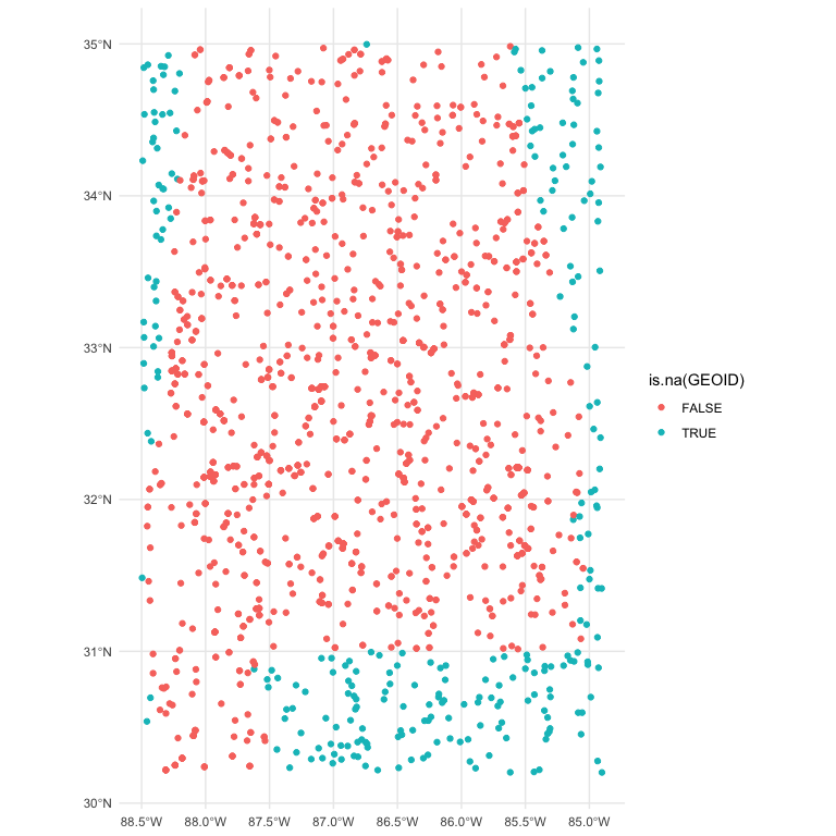
If a point is not in the polygon database, an NA is returned.

library(ggplot2)

res |> 
  ggplot(aes(color = is.na(GEOID))) +
  geom_sf() +
  theme_minimal()

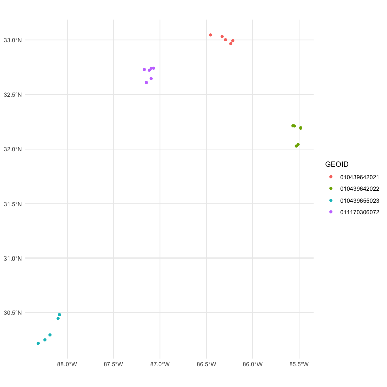
# whoops is the join working?

ids <- res |> 
  select(GEOID) |> 
  count(GEOID, sort = TRUE) |> 
  slice(7:10) |> 
  pull(GEOID)

res |> 
  filter(GEOID %in% ids) |> 
  ggplot(aes(color = GEOID)) +
  geom_sf() +
  theme_minimal()

API

Do this as an API.

TODO: issue is that call_that generated API can’t find the plumber.R But API works.

library(callthat)
library(httr2)

api_conn <- call_that_plumber_start(
  system.file("plumber/sample-api", package = "bullseye")
)

df <- data.frame(
  id = c(1, 2),
  lat = c(31.58037, 33.98386),
  lng = c(-87.51496, -86.36208)
)

# Create and tailor the request

# req <- request(api_conn) |>
#   req_method("POST") |>
#   req_body_json(data = df) |>
#   req_headers("Content-Type" = "application/json")

# this does the above, but with call_that
post_coord <- call_that_api_post(
      api_conn, 
      endpoint = "compute", 
      body = jsonlite::toJSON(df)
)



# Perform the request

# req |>
#   req_perform() |>
#   resp_body_json()

post_coord |> 
  resp_body_json()

call_that_plumber_stop(api_conn)

Deploy

But that’s not all! bullseye comes with a Dockerfile. So just navigate to the project folder, and build and run.

docker build -t bullseye_image .
docker run --rm -p 8000:8000 bullseye_image