- 1. Methodology
- 2. Installation
- 3. Usage
- 4. Experiments
To accelerate CNN inference, existing deep learning frameworks focus on optimizing intra-operator parallelization.
However, a single operator can no longer fully utilize the available parallelism given the rapid advances in high-performance hardware,
resulting in a large gap between the peak performance and the real performance.
This performance gap is more severe under smaller batch sizes.
In this work, we extensively study the parallelism between operators and propose Inter-Operator Scheduler (IOS) to automatically schedule the execution of multiple operators in parallel.
IOS utilizes dynamic programming to find a scheduling policy specialized for the target hardware.
IOS consistently outperforms state-of-the-art libraries (e.g., TensorRT) by 1.1 to 1.5x on modern CNN benchmarks.
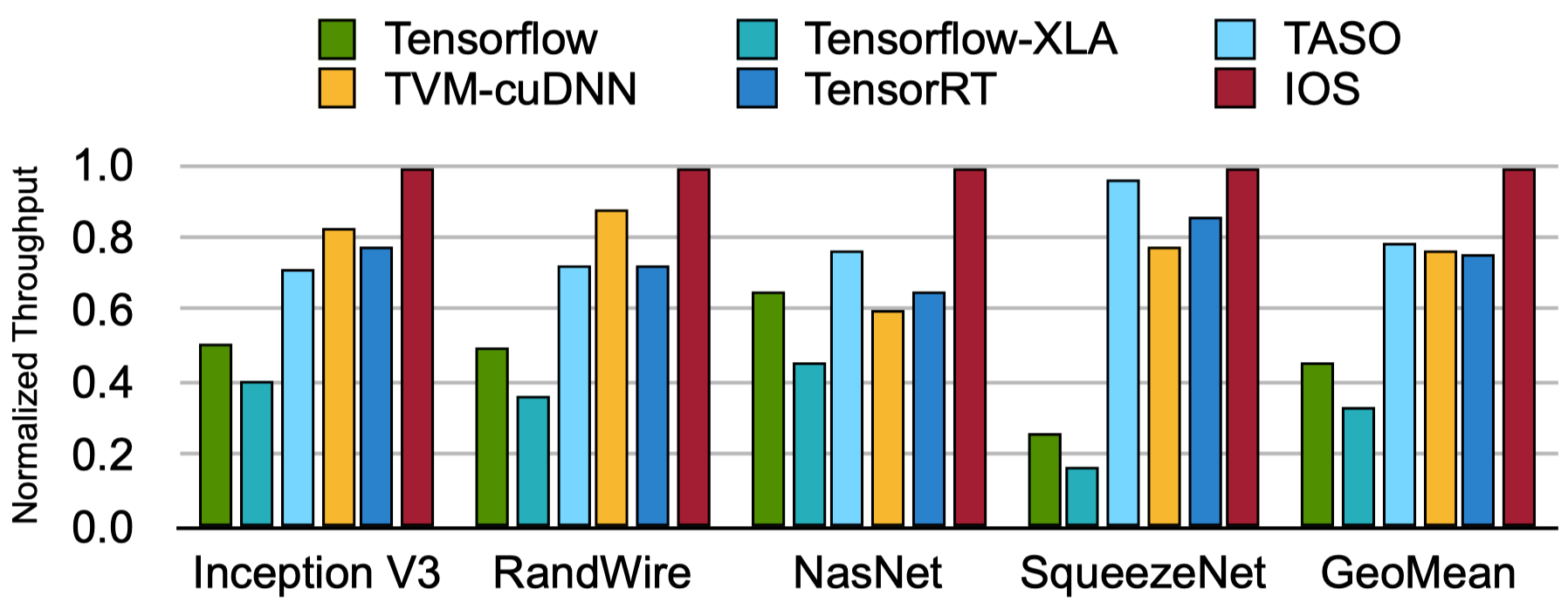
End-to-end performance comparison of different frameworks across different CNNs on batch size one. The throughput is normalized to the best one for each model.
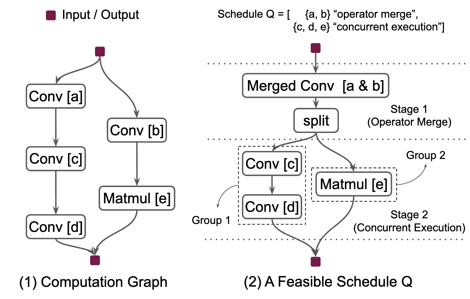
IOS partitions given computation graph into multiple stages . Each stage has a parallelization strategy.
As shown in the above figure, the computation graph in (1) is partitioned into two stages in (2). The first stage contains operator a and b, and the second stage contains operator c, d, and e. The first stage merge the two convolutions and the second stage concurrent execute the independent groups of operators. Such an partition with the parallelization strategy for each stage in the partition is called a schedule for the computation graph in IOS.The number of feasible schedules for a computation graph grows exponentially with respect with the number of operators in the computation graph. It is challenging to find an highly optimized schedule of given computation graph within reasonable time. IOS takes advantage of the common sub-schedules among different schedules and utilizes dynamic programming technique to find an highly optimized schedule for given computation graph. For more details, please refer the Methods section in our paper.
Please follow this section to build IOS from source code.
- CMake 3.10 or higher
- CUDA Toolkit 10.0 or higher
- cuDNN 7.6.5 or higher
To get started, clone the IOS source code from Github.
git clone https://github.com/mit-han-lab/inter-operator-scheduler.git ios
cd ios
Then build the IOS runtime:
mkdir build
cd build;
cmake ..; make -j4
cd ..Once the IOS runtime has been built, run following commands to install the IOS python package.
cd python;
python setup.py install --userIOS optimizes user-defined computation graph and does inference on IOS runtime. The following code snip shows how to use IOS, in which user
- defines the computation graph first,
- then optimizes the execution schedule,
- and executes the network on IOS runtime at last.
import numpy as np
import ios

def sample_network():
    v = ios.placeholder(output_shape=(375, 15, 15))
    block = ios.Block(enter_node=v.node)
    v1 = ios.conv2d(block, inputs=[[v]], out_channels=375, kernel=(3, 3), stride=(1, 1), padding=(1, 1), act='relu')
    v2 = ios.conv2d(block, inputs=[[v]], out_channels=750, kernel=(3, 3), stride=(1, 1), padding=(1, 1), act='relu')
    v3 = ios.conv2d(block, inputs=[[v]], out_channels=375, kernel=(3, 3), stride=(1, 1), padding=(1, 1), act='relu')
    v1 = ios.conv2d(block, inputs=[[v1]], out_channels=750, kernel=(3, 3), stride=(1, 1), padding=(1, 1), act='relu')
    out = ios.identity(block, inputs=[[v1], [v2], [v3]], is_exit=True)  # concat v1, v2, and v3
    graph = ios.Graph(name="demo", input=v.node, blocks=[block])
    graph.init_weights()
    return graph

# define computation graph
graph = sample_network()

# optimize execution schedule
optimized_graph = ios.optimize(graph, batch_size=1, opt_type='dp_parallel', compute_weight=True)

# measure latency
graph.sequential_schedule()
seq_latency, stage_latency = ios.ios_runtime.graph_latency(graph, batch_size=1, repeat=6, profile_stage=True)
print(graph)
print(f'Sequential schedule: {np.mean(seq_latency):.3f} ms')
print(f'      Stage latency: {np.mean(np.array(stage_latency).reshape(6, -1), axis=0)}\n')

opt_latency, stage_latency = ios.ios_runtime.graph_latency(optimized_graph, batch_size=1, repeat=6, profile_stage=True)
print(optimized_graph)
print(f'Optimized schedule: {np.mean(opt_latency):.3f} ms')
print(f'     Stage latency: {np.mean(np.array(stage_latency).reshape(6, -1), axis=0)}')

# inference on ios runtime
dummy_inputs = np.random.randn(1, 375, 15, 15)
output = ios.ios_runtime.graph_inference(optimized_graph, batch_size=1, input=dummy_inputs)
An output of this program:
Sequential(
  [1]Conv2d(0)
  [2]Conv2d(0)
  [3]Conv2d(0)
  [4]Conv2d(1)
  [5]Concat(4,2,3)
)
Sequential schedule: 0.486 ms
      Stage latency: [0.11070578 0.12603733 0.10604089 0.12549689 0.01794844]

Sequential(
  Parallel(
    [1]Conv2d(0)
    [2]Conv2d(0)
  )
  Parallel(
    [4]Conv2d(1)
    [3]Conv2d(0)
  )
  [5]Concat(4,2,3)
)
Optimized schedule: 0.333 ms
     Stage latency: [0.16145067 0.15448178 0.01732267]
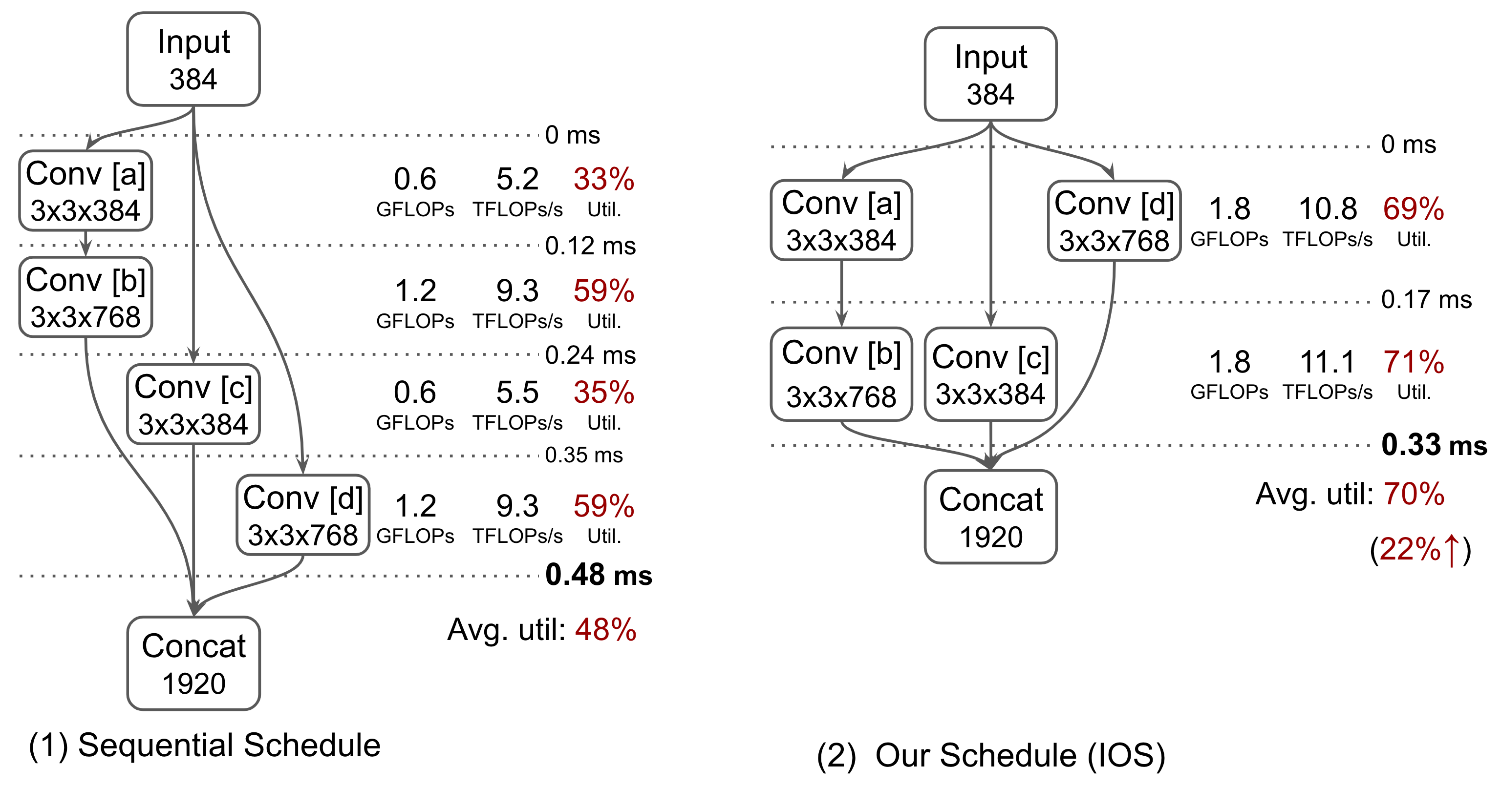
The following figure shows the sequential schedule and our schedule of the defined sample network.
The following parts shows the commands to reproduce all experiments and ablation study.
In this experiment, we compared IOS with different frameworks as follows
All experiments all conducted under following environment.
- Python 3.7
- NVIDIA Driver 450.51.05
- CUDA Toolkit 10.2
- CUDNN 7.6.5
- TensorRT 7.0.0.11
- TVM v0.6
- TASO v1.0
- Tensorflow 2.3
- PyTorch 1.6.0
The perquisites for each experiment(from 1 to 7) are
- Experiment 1, 3, 4, 5 do not require any other frameworks/libraries
- Experiment 2 requires TensorRT, TVM, TASO, Tensorflow, and PyTorch (you can ignore any of them if you do not want to compare IOS with it)
- Experiment 6 requires TensorRT (you can ignore it if you only compare Sequential schedule and IOS optimized schedule)
- Experiment 7 reqruies TVM
We recommend you reproduce the experiments in a conda environment:
conda create -n ios python=3.7
conda activate ios- Download the TensorRT from NVIDIA website. We recommend to download the tar archive.
- Extract the TensorRT archive to somewhere. Please use the tar.gz file you downloaded.
tar xvzf ~/Downloads/TensorRT-7.0.0.11.Ubuntu-18.04.x86_64-gnu.cuda-10.2.cudnn7.6.tar.gz /path/to/unarchive - Configure the
config.cmakefile in ios root directory. Changeset(USE_TRT OFF)toset(USE_TRT /path/to/unarchive/TensorRT-TensorRT-7.0.0.11). - Rebuild IOS runtime and TRT runtime, and reinstall IOS python package:
cd /path/to/ios;
mkdir -p build; cd build; cmake ..; make -j4; cd ..
cd python; python setup.py install; cd ..
- Add
/path/to/tensorrt/libto the end ofLD_LIBRARY_PATH.export LD_LIBRARY_PATH=$LD_LIBRARY_PATH:/path/to/TensorRT-x.x.x.x/lib
Now we finished the installation of TensorRT runtime in IOS. We can infer the IOS computation graph and measure its latency using ios.trt_runtime module as follows
import numpy as np
import ios
graph = ios.models.inception_v3()
# measure latency
latency = ios.trt_runtime.graph_latency(graph, batch_size=1, repeat=5)
# inference
outputs = ios.trt_runtime.graph_inference(graph, batch_size=1, input=np.random.randn(1, 3, 299, 299))
Module ios.trt_runtime converts the IOS computation graph ios.Graph to the corresponding TensorRT network, measures the latency and executes the network using TensorRT library.
Please refer the TVM installation guide for the instructions to install TVM. Because we need to customize the installation configuration (step 3 bellow), we put the installation commands here for simplicity.
- Clone the TVM source code from Github.
git clone https://github.com/apache/incubator-tvm.git tvm
cd tvm;
git checkout v0.6  # you can change v0.6 to v0.7 or higher to use higher version of TVM
git submodule update --resursive --init
mkdir build; cp cmake/config.cmake build;
- Install
llvmbysudo apt install llvm. - Configure
build/config.cmake.- Replace
set(USE_CUDA OFF)byset(USE_CUDA ON)orset(USE_CUDA /path/to/a/specific/cuda_toolkit). - Replace
set(USE_CUDNN OFF)toset(USE_CUDNN ON). - Replace
set(USE_LLVM OFF)toset(USE_LLVM ON).
- Replace
- Build and Install TVM.
cd build; cmake ..; make -j8; cd ..;
cd python; python setup.py install --user; cd ..;
cd topi/python; python setup.py install --user; cd ../.. # for tvm v0.6, ignore for tvm v0.7 or higher
- Validate that you have successfully installed TVM by
import tvm
print(tvm.__version__)
Please refer the TASO installation guide for the instructions to install TASO.
pip install tensorflowconda install pytorch torchvision -c pytorchBecause modern GPU can adjust the execution clock rate dynamically to reduce energy consumption when the device is not busy. We can lock the clock rate to make the experiment results more accurate and consistent. Before conducting the experiments, run the following command (need sudo-privilege).
sudo nvidia-smi --lock-gpu-clocks=MIN_CLOCK,MAX_CLOCKThis command lock the gpu clocks in the specified range [MIN_CLOCK, MAX_CLOCK].
In our experiments, we set both MIN_CLOCK and MAX_CLOCK to 1530,
which is the maximum clock rate NVIDIA Tesla V100 SXM2 supports.
You can use the following command to query the clock rates supported by your NVIDIA GPU,
nvidia-smi --query --display=SUPPORTED_CLOCKSand use this command to watch the current GPU clock rate:
watch nvidia-smi --query --display=CLOCKAfter the experiments, you can run the following command to reset your GPU clock
sudo nvidia-smi --reset-gpu-clocksRefer here and man nvidia-smi for more information.
Once the experiment environment has been setup, we can conduct the 7 experiments and ablation study in the paper. All the experiments results in the paper (shown in the figure) are the average of five repeated experiment results. To save the time, the code in this section only conducts one time. All the differences between the output and numbers in paper are within the allowable error range.
This experiment compare the following schedules: Sequential, Greedy, IOS-Merge, IOS-Parallel, and IOS-Both. For fair comparison, all schedules are executed in the same execution engine (IOS runtime).
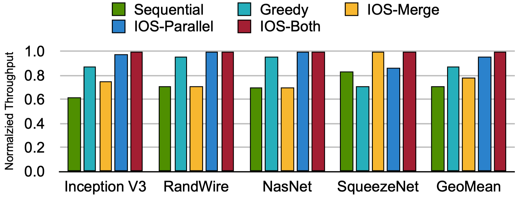
End-to-end performance comparison of different schedules across different CNNs on batch size one. The throughput is normalized to the best one for each model.
The following table gives the latency (ms) for each model and schedule.
| Schedule | Sequential | Greedy | IOS-Merge | IOS-Parallel | IOS-Both |
|---|---|---|---|---|---|
| Inception V3 | 6.51 | 4.62 | 5.39 | 4.11 | 4.03 |
| RandWire | 8.49 | 6.27 | 8.54 | 6.02 | 6.02 |
| NasNet | 22.95 | 16.78 | 22.94 | 16.04 | 16.04 |
| SqueezeNet | 0.86 | 0.98 | 0.74 | 0.82 | 0.73 |
| GeoMean | 5.74 | 4.67 | 5.28 | 4.24 | 4.11 |
Command:
cd experiments/latency; sh run_expr_schedules.sh; cd ../..Key output:
Model: inception_v3 | Optimization: Sequential      | Batchsize: 1  | Optimization cost: 0 sec    | Latency: 6.25 ms
Model: inception_v3 | Optimization: Greedy          | Batchsize: 1  | Optimization cost: 0 sec    | Latency: 4.62 ms
Model: inception_v3 | Optimization: IOS-Merge       | Batchsize: 1  | Optimization cost: 1 sec    | Latency: 5.13 ms
Model: inception_v3 | Optimization: IOS-Parallel    | Batchsize: 1  | Optimization cost: 48 sec   | Latency: 4.06 ms
Model: inception_v3 | Optimization: IOS-Both        | Batchsize: 1  | Optimization cost: 48 sec   | Latency: 3.94 ms
Model: randwire     | Optimization: Sequential      | Batchsize: 1  | Optimization cost: 0 sec    | Latency: 8.53 ms
Model: randwire     | Optimization: Greedy          | Batchsize: 1  | Optimization cost: 0 sec    | Latency: 6.27 ms
Model: randwire     | Optimization: IOS-Merge       | Batchsize: 1  | Optimization cost: 3 sec    | Latency: 8.58 ms
Model: randwire     | Optimization: IOS-Parallel    | Batchsize: 1  | Optimization cost: 4386 sec | Latency: 5.80 ms
Model: randwire     | Optimization: IOS-Both        | Batchsize: 1  | Optimization cost: 4407 sec | Latency: 5.78 ms
Model: nasnet       | Optimization: Sequential      | Batchsize: 1  | Optimization cost: 0 sec    | Latency: 23.02 ms
Model: nasnet       | Optimization: Greedy          | Batchsize: 1  | Optimization cost: 0 sec    | Latency: 16.60 ms
Model: nasnet       | Optimization: IOS-Merge       | Batchsize: 1  | Optimization cost: 63 sec   | Latency: 23.06 ms
Model: nasnet       | Optimization: IOS-Parallel    | Batchsize: 1  | Optimization cost: 3591 sec | Latency: 15.87 ms
Model: nasnet       | Optimization: IOS-Both        | Batchsize: 1  | Optimization cost: 3653 sec | Latency: 15.85 ms
Model: squeezenet   | Optimization: Sequential      | Batchsize: 1  | Optimization cost: 0 sec    | Latency: 0.89 ms
Model: squeezenet   | Optimization: Greedy          | Batchsize: 1  | Optimization cost: 0 sec    | Latency: 0.98 ms
Model: squeezenet   | Optimization: IOS-Merge       | Batchsize: 1  | Optimization cost: 0 sec    | Latency: 0.68 ms
Model: squeezenet   | Optimization: IOS-Parallel    | Batchsize: 1  | Optimization cost: 1 sec    | Latency: 0.86 ms
Model: squeezenet   | Optimization: IOS-Both        | Batchsize: 1  | Optimization cost: 1 sec    | Latency: 0.68 ms
This experiment compare IOS with other cuDNN-based frameworks/libraries: Tensorflow, TVM-cuDNN, TASO, and TensorRT.
TVM-cuDNN is the TVM framework, but convolution uses the cuDNN kernel (target = 'cuda -libs=cudnn').

End-to-end performance comparison of different frame-works across different CNNs on batch size one. The throughput is normalized to the best one for each model.
The following table gives the latency (ms) for each model and framework/library.
| Frameworks | Tensorflow | Tensorflow-XLA | TASO | TVM-cuDNN | TensorRT | IOS |
|---|---|---|---|---|---|---|
| Inception V3 | 7.95 | 9.95 | 5.70 | 4.88 | 5.21 | 4.03 |
| RandWire | 12.06 | 16.61 | 8.42 | 6.86 | 8.33 | 6.02 |
| NasNet | 24.73 | 34.66 | 21.29 | 26.87 | 24.66 | 16.04 |
| SqueezeNet | 2.63 | 4.08 | 0.82 | 0.90 | 0.80 | 0.73 |
| GeoMean | 8.88 | 12.36 | 5.37 | 5.54 | 5.41 | 4.11 |
Command:
cd experiments/latency; sh run_expr_frameworks.sh; cd ../..Key output:
Model: inception_v3 | Optimization: Tensorflow      | Batchsize: 1  | Optimization cost: 4 sec    | Latency: 7.70 ms
Model: inception_v3 | Optimization: Tensorflow-XLA  | Batchsize: 1  | Optimization cost: 6 sec    | Latency: 9.37 ms
Model: inception_v3 | Optimization: TASO            | Batchsize: 1  | Optimization cost: 50 sec   | Latency: 5.47 ms
Model: inception_v3 | Optimization: TVM-cuDNN       | Batchsize: 1  | Optimization cost: 29 sec   | Latency: 4.88 ms
Model: inception_v3 | Optimization: TensorRT        | Batchsize: 1  | Optimization cost: 17 sec   | Latency: 4.77 ms
Model: randwire     | Optimization: Tensorflow      | Batchsize: 1  | Optimization cost: 5 sec    | Latency: 11.31 ms
Model: randwire     | Optimization: Tensorflow-XLA  | Batchsize: 1  | Optimization cost: 12 sec   | Latency: 14.86 ms
Model: randwire     | Optimization: TASO            | Batchsize: 1  | Optimization cost: 5222 sec | Latency: 8.65 ms
Model: randwire     | Optimization: TVM-cuDNN       | Batchsize: 1  | Optimization cost: 28 sec   | Latency: 6.82 ms
Model: randwire     | Optimization: TensorRT        | Batchsize: 1  | Optimization cost: 108 sec  | Latency: 7.93 ms
Model: nasnet       | Optimization: Tensorflow      | Batchsize: 1  | Optimization cost: 8 sec    | Latency: 24.14 ms
Model: nasnet       | Optimization: Tensorflow-XLA  | Batchsize: 1  | Optimization cost: 19 sec   | Latency: 32.47 ms
Model: nasnet       | Optimization: TASO            | Batchsize: 1  | Optimization cost: 36 sec   | Latency: 21.26 ms
Model: nasnet       | Optimization: TVM-cuDNN       | Batchsize: 1  | Optimization cost: 54 sec   | Latency: 26.83 ms
Model: nasnet       | Optimization: TensorRT        | Batchsize: 1  | Optimization cost: 246 sec  | Latency: 24.38 ms
Model: squeezenet   | Optimization: Tensorflow      | Batchsize: 1  | Optimization cost: 2 sec    | Latency: 2.59 ms
Model: squeezenet   | Optimization: Tensorflow-XLA  | Batchsize: 1  | Optimization cost: 4 sec    | Latency: 3.71 ms
Model: squeezenet   | Optimization: TASO            | Batchsize: 1  | Optimization cost: 3 sec    | Latency: 0.82 ms
Model: squeezenet   | Optimization: TVM-cuDNN       | Batchsize: 1  | Optimization cost: 11 sec   | Latency: 0.88 ms
Model: squeezenet   | Optimization: TensorRT        | Batchsize: 1  | Optimization cost: 8 sec    | Latency: 0.81 ms
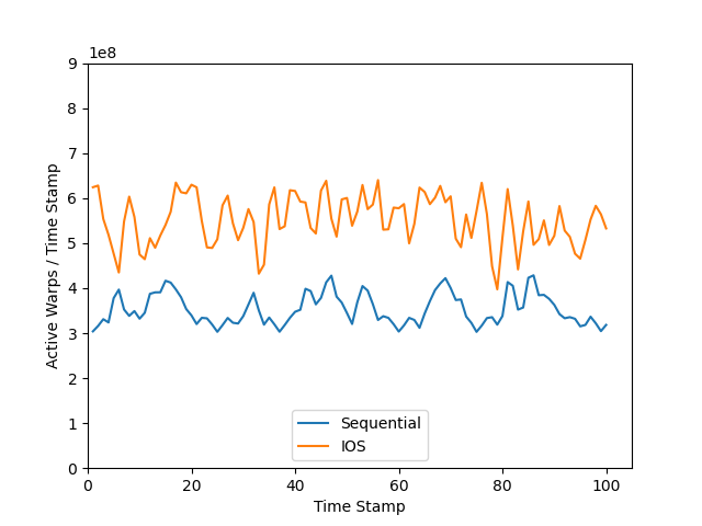
This experiment profiles the active warps of sample network defined in Usage under Sequential schedule and IOS-Both schedule. The NVIDIA CUDA Profiling Tools Interface (CUPTI) is used to profile.
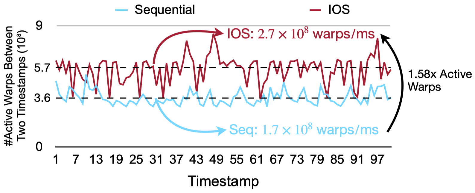
The profiling of active warps for the sample network defined in experiments/sample.py.
Active warps
indicates the number of actually executed instructions (1 warp = 32 inst.) on the device and can be used to show the device utilization.
There is about 2.1 ms between two timestamps on average.
IOS achieves higher device utilization (active warps/ms) than the sequential schedule.
Command:
cd experiments/utilization; sh run_expr_utilization.sh; cd ../..Above command would generate a plot image named active_warps.png, which can reflect the real device utilization.
Here is a sample of the figure:
IOS support specialized scheduling for different devices and different batch sizes.

Latency (ms) of specialized schedules for batch size 1, 32 and 128, and specialized schedules for NVIDIA Tesla K80 and V100. The best performance is achieved when the schedule is specialized for each batch size and device. Each row is the batch size or device that the model is executed on. Each column is the batch size or device that IOS optimized for. InceptionV3 is used as benchmark.
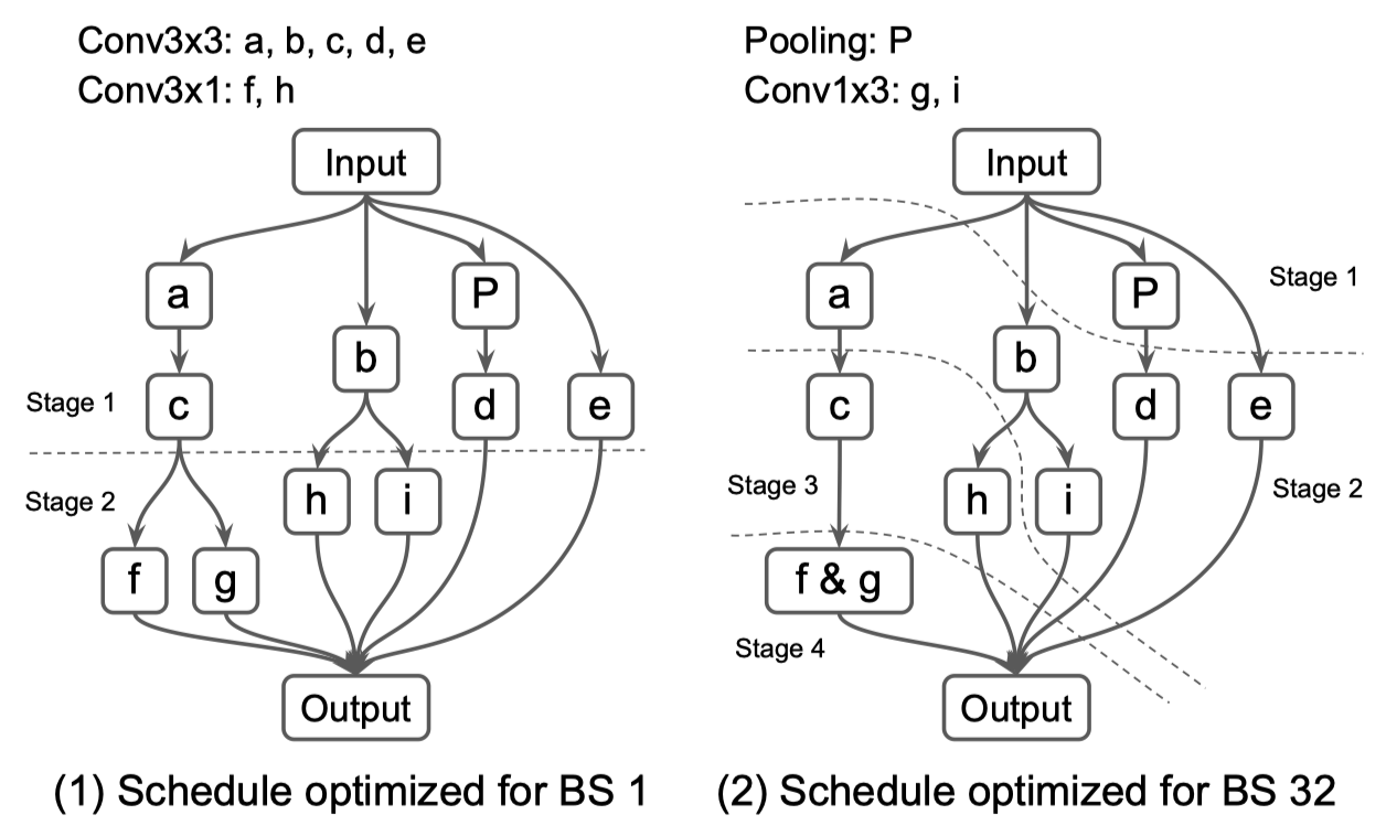
The schedule found by IOS for the last block of Inception V3. Operator a-e are convolution operator while operator P is the pooling operator. Schedule (1) and (2) are optimized for batch size 1 and 32 respectively. In schedule (1), there are two stages while in schedule (2) there are 4 stages. Schedule (1) is 28% faster than schedule (2) on batch size 1. Schedule (2) is 8% faster than schedule (1) on batch size 32.
We first optimize for different batch sizes (1, 32, and 128) to get the schedule specialized for different batch sizes (for your simplicity, we have put the schedules we got in the schedules directory).
Then we execute the network Inception V3 with different batch sizes and specialized schedules (there are 25 combinations, 5 by 5).
To explore the specialization for different batch sizes, run the following command:
cd experiments/specialization; sh run_expr_spec_batchsize.sh; cd ../..Key output:
Optimized for BS 1    Execute with BS 1    Latency: 4.04 ms
Optimized for BS 1    Execute with BS 32   Latency: 29.21 ms
Optimized for BS 1    Execute with BS 128  Latency: 105.87 ms
Optimized for BS 32   Execute with BS 1    Latency: 4.45 ms
Optimized for BS 32   Execute with BS 32   Latency: 27.62 ms
Optimized for BS 32   Execute with BS 128  Latency: 103.58 ms
Optimized for BS 128  Execute with BS 1    Latency: 4.58 ms
Optimized for BS 128  Execute with BS 32   Latency: 27.85 ms
Optimized for BS 128  Execute with BS 128  Latency: 102.96 ms
To explore the specialization for different devices, we need a different GPU device. In our experiment, we take NVIDIA Tesla K80 as the second device.
We first optimize the network on different devices to get the specialized schedules (we also put them in schedules directory).
Then we execute the network with different specialized schedules on the two devices (there are 4 combinations, 2 by 2).
Run the following commands on NVIDIA Tesla V100 and K80 with DEVICE=v100 and DEVICE=k80, respectively.
cd experiments/specialization; sh run_expr_spec_device.sh DEVICE; cd ../..Key output log when executed on V100 and DEVICE=v100:
Run on v100
Optimized for k80   Execute with v100  Latency: 4.42 ms
Optimized for v100  Execute with v100  Latency: 4.02 ms
Key output log when executed on K80 and DEVICE=k80:
Run on k80
Optimized for k80   Execute with k80   Latency: 13.93 ms
Optimized for v100  Execute with k80   Latency: 14.64 ms
(Because NVIDIA Tesla K80 can not lock the gpu clock, you need to warmup the gpu to make it working with highest clock rate to get above result.)
Experiments show that specialized scheduling is beneficial.
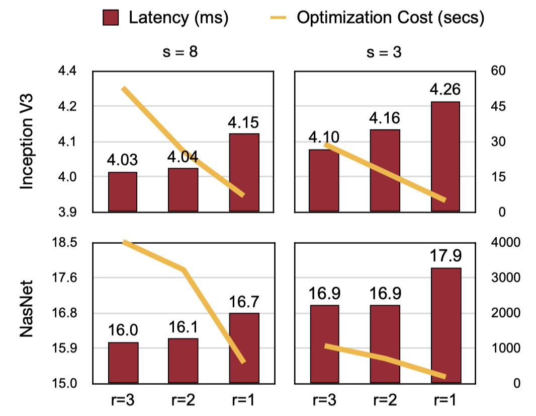
To allow users to trade off the search time and optimized schedule latency, we introduce the schedule pruning strategy to reduce the search time. This experiment shows the trade-off between the search time and schedule latency.
Command:
cd experiments/latency; sh run_expr_prune.sh; cd ../..Key output:
Model: inception_v3 | Optimization: IOS-Both(r=1, s=3)   | Batchsize: 1  | Optimization cost: 5 sec    | Latency: 4.22 ms
Model: inception_v3 | Optimization: IOS-Both(r=1, s=8)   | Batchsize: 1  | Optimization cost: 7 sec    | Latency: 4.06 ms
Model: inception_v3 | Optimization: IOS-Both(r=2, s=3)   | Batchsize: 1  | Optimization cost: 17 sec   | Latency: 4.02 ms
Model: inception_v3 | Optimization: IOS-Both(r=2, s=8)   | Batchsize: 1  | Optimization cost: 25 sec   | Latency: 3.99 ms
Model: inception_v3 | Optimization: IOS-Both(r=3, s=3)   | Batchsize: 1  | Optimization cost: 29 sec   | Latency: 3.99 ms
Model: inception_v3 | Optimization: IOS-Both(r=3, s=8)   | Batchsize: 1  | Optimization cost: 43 sec   | Latency: 3.96 ms
Model: nasnet       | Optimization: IOS-Both(r=1, s=3)   | Batchsize: 1  | Optimization cost: 137 sec  | Latency: 17.54 ms
Model: nasnet       | Optimization: IOS-Both(r=1, s=8)   | Batchsize: 1  | Optimization cost: 492 sec  | Latency: 16.54 ms
Model: nasnet       | Optimization: IOS-Both(r=2, s=3)   | Batchsize: 1  | Optimization cost: 360 sec  | Latency: 16.85 ms
Model: nasnet       | Optimization: IOS-Both(r=2, s=8)   | Batchsize: 1  | Optimization cost: 2648 sec | Latency: 16.09 ms
Model: nasnet       | Optimization: IOS-Both(r=3, s=3)   | Batchsize: 1  | Optimization cost: 641 sec  | Latency: 16.73 ms
Model: nasnet       | Optimization: IOS-Both(r=3, s=8)   | Batchsize: 1  | Optimization cost: 3412 sec | Latency: 15.91 ms
IOS can achieve consistent improvement for different batch sizes. In this experiment, we measure the latency of Inception V3 on batch size 1, 16, 32, 64, 128. Experiment result show that IOS consistently outperforms TensorRT in terms of throughput.
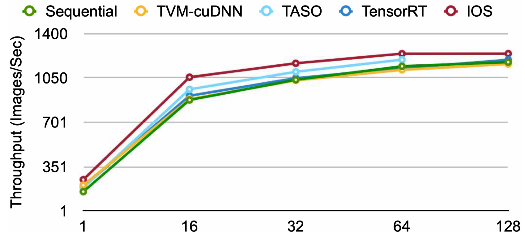
The throughput comparison of Sequential schedule, TensorRT and IOS on batch size 1, 16, 32, 64 and 128 for Inception V3.
Command:
cd experiments/latency; sh run_expr_batchsize.sh; cd ../..Key output:
Model: inception_v3 | Optimization: Sequential      | Batchsize: 1  | Optimization cost: 0 sec    | Latency: 6.20 ms
Model: inception_v3 | Optimization: TensorRT        | Batchsize: 1  | Optimization cost: 17 sec   | Latency: 4.82 ms
Model: inception_v3 | Optimization: IOS-Both        | Batchsize: 1  | Optimization cost: 48 sec   | Latency: 3.94 ms
Model: inception_v3 | Optimization: Sequential      | Batchsize: 16 | Optimization cost: 0 sec    | Latency: 17.95 ms
Model: inception_v3 | Optimization: TensorRT        | Batchsize: 16 | Optimization cost: 8 sec    | Latency: 17.82 ms
Model: inception_v3 | Optimization: IOS-Both        | Batchsize: 16 | Optimization cost: 131 sec  | Latency: 15.17 ms
Model: inception_v3 | Optimization: Sequential      | Batchsize: 32 | Optimization cost: 0 sec    | Latency: 30.54 ms
Model: inception_v3 | Optimization: TensorRT        | Batchsize: 32 | Optimization cost: 9 sec    | Latency: 29.97 ms
Model: inception_v3 | Optimization: IOS-Both        | Batchsize: 32 | Optimization cost: 207 sec  | Latency: 27.00 ms
Model: inception_v3 | Optimization: Sequential      | Batchsize: 64 | Optimization cost: 0 sec    | Latency: 55.67 ms
Model: inception_v3 | Optimization: TensorRT        | Batchsize: 64 | Optimization cost: 11 sec   | Latency: 56.25 ms
Model: inception_v3 | Optimization: IOS-Both        | Batchsize: 64 | Optimization cost: 368 sec  | Latency: 51.11 ms
Model: inception_v3 | Optimization: Sequential      | Batchsize: 128 | Optimization cost: 0 sec    | Latency: 108.55 ms
Model: inception_v3 | Optimization: TensorRT        | Batchsize: 128 | Optimization cost: 16 sec   | Latency: 106.84 ms
Model: inception_v3 | Optimization: IOS-Both        | Batchsize: 128 | Optimization cost: 711 sec  | Latency: 102.74 ms
AutoTVM is specialized for improvement the efficiency of the kernel by searching a highly optimized schedule for the kernel itself.
Current IOS is implemented based on vendor-provided library cuDNN.
We compare both of them to give us more insight about the intra- and inter-operator parallelism.
Because AutoTVM is time consuming (it takes 26 hours on a 8-V100 server to optimize the four benchmark networks), we provide the schedule configs tuned by us in tvm_schedule_configs directory.
You can use these configs directly to reproduce the experiments.
Please note that these schedule configs are optimized for NVIDIA Tesla V100 SXM2 with driver 450.51.05 and cuda toolkit 10.2 using TVM v0.6.
If you want to tune the network by yourself, just delete the ./schedules directory and we would tune the network using TVM and store the tuned schedule configs in ./tvm_schedule_configs automatically.
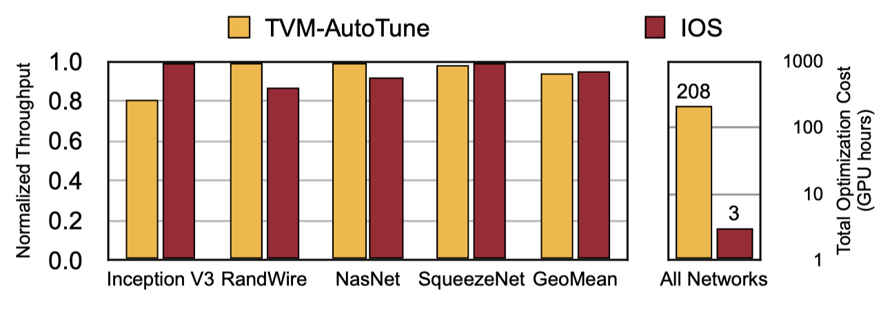
End-to-end performance comparison between TVM-AutoTune and IOS. TVM-AutoTune and IOS are orthogonal because TVM focuses on the intra-operator parallelism while IOS focuses on inter-operator parallelism. They can be combined to further boost the inference performance. The optimization cost of IOS is two orders of magnitude less than TVM.
Command:
cd experiments/latency; sh run_expr_autotvm.sh; cd ../..Key output:
Model: inception_v3 | Optimization: TVM-AutoTune    | Batchsize: 1  | Optimization cost: 21 sec   | Latency: 4.95 ms
Model: randwire     | Optimization: TVM-AutoTune    | Batchsize: 1  | Optimization cost: 26 sec   | Latency: 5.26 ms
Model: nasnet       | Optimization: TVM-AutoTune    | Batchsize: 1  | Optimization cost: 28 sec   | Latency: 14.67 ms
Model: squeezenet   | Optimization: TVM-AutoTune    | Batchsize: 1  | Optimization cost: 13 sec   | Latency: 0.75 ms
(The Optimization cost shown in the output is the time used to compile the network and measure latency, which does not include the time for auto-tuning, because the pre-tuned configs are used.
It takes about 26 hours on a 8-V100 server to tune the four networks.)
