A Fortran code to simulation the non-adiabatic Molecular Dynamics in the solid state Materials. We using a linear vibroninc coupling model implementation of Tully's Fewest Switches Surface Hopping (FSSH) for model problems including a propagator and an implementation of Tully's model problems described in Tully, J.C. J. Chem. Phys. (1990) 93 1061.
The code are writen in Fortran, and need MKL Fortran 95 library. To compiler the code, do as follwing step.
module load compiler/intel/2020.4.302
tar -zxvf lvcsh.tar.gz
cd LVCSH
cd make
make
cd ../make_complex
make The the code use the EPW output file as main input file. Now only the version of V.6.8 of Quantum_Espresso be support and need to change the EPW source code and recompile to print out the gmnvkq and vmef in complex formated.
cp LVCSH/docs/QE_change_code/v6.8/* qe-6.8/EPW/src
cd qe-6.8
make epw-
make a work directory (Carbyne)
-
In work directory do epw calculate, to get the electron-phonon coupling matrix. the dir structure as follow
                 (work directory)
     ___________________|_______________________________
    |       |       |     |         |          |        |
  relax   pseudo   scf   dos     phonon       epw      LVCSH
计算电声耦合项的步骤如下所示。在不同的目录下面进行结构优化、自洽计算、声子谱计算和电声耦合计算
2.1 进入relax目录,创建vc-relax.in 进行晶格结构优化。对于参数的设置,
etot_conv_thr,forc_conv_thr,conv_thr和press_conv_thr的精度需要设置的比较高,需要用于后续计算phonon. 在该案例中收敛判据可能不够,在实际的计算中,应该根据需要进行设置。vc-relax.in &CONTROL calculation = "vc-relax" restart_mode = "from_scratch" prefix = "carbyne" outdir = "./" pseudo_dir = "./pseudo/" verbosity = "high" tprnfor = .true. tstress = .true. etot_conv_thr = 1.0d-5 forc_conv_thr = 1.0d-4 / &SYSTEM ibrav = 0 nat = 2 ntyp = 1 !nbnd = 16 occupations = 'fixed' ! occupations = "smearing" ! smearing = "cold" ! degauss = 1.0d-2 ecutwfc = 50 ecutrho = 400 / &ELECTRONS conv_thr = 1.000e-7 electron_maxstep = 200 mixing_beta = 7.00000e-01 startingpot = "atomic" startingwfc = "atomic+random" / &IONS ion_dynamics = "bfgs" / &CELL cell_dofree = "x" cell_dynamics = "bfgs" press_conv_thr = 0.02 / K_POINTS {automatic} 200 1 1 0 0 0 ATOMIC_SPECIES C 12.01070 C.pbe-n-kjpaw_psl.1.0.0.UPF CELL_PARAMETERS (angstrom) 2.565602620 0.000000000 0.000000000 0.000000000 10.000000000 0.000000000 0.000000000 0.000000000 10.000000000 ATOMIC_POSITIONS (angstrom) C 0.0002913894 5.0000000000 5.0000000000 C 1.2644833916 5.0000000000 5.0000000000
采用下面命令查看计算过程中的受力情况已经压力张量和晶格常数变化情况
cat vc-relax.out |grep -A 12 "Total force ="
计算结束后,使用下面命令得到优化后的结果
grep -B 30 "Begin final coordinates" vc-relax.outawk '/Begin final coordinates/,/End final coordinates/{print $0}' vc-relax.outBegin final coordinates new unit-cell volume = 1731.62982 a.u.^3 ( 256.60106 Ang^3 ) density = 0.15545 g/cm^3 CELL_PARAMETERS (angstrom) 2.566010647 0.000000000 0.000000000 0.000000000 10.000000000 0.000000000 0.000000000 0.000000000 10.000000000 ATOMIC_POSITIONS (angstrom) C 0.0019333750 5.0000000000 5.0000000000 C 1.2630425527 5.0000000000 5.0000000000 End final coordinates2.2
cp vc-relax.in relax.in将上面优化得到的CELL_PARAMETERS和ATOMIC_POSITIONS结果在relax.in中进行修改,并修改为calculation = "relax", 将&CELL /部分注释掉。再对原子位置进行优化。计算完成后,运行下列命令查看优化过程中原子受力情况和得到优化后的原子位置。cat relax.out |grep -A 12 "Total force ="
grep -B 30 "Begin final coordinates" vc-relax.outawk '/Begin final coordinates/,/End final coordinates/{print $0}' relax.out得到如下结果:
Begin final coordinates

 ATOMIC_POSITIONS (angstrom)
 C             0.0019333750        5.0000000000        5.0000000000
 C             1.2630425527        5.0000000000        5.0000000000
 End final coordinates
2.3
cp relax.in scf.in将上面的原子位置(ATOMIC_POSITIONS)结果在scf.in文件中进行修改。修改calculation = "scf"将&IONS /部分注释掉。mkdir ../scf并将修改后的scf.in文件复制到../scf中,修改scf.in中的outdir= './'进行自洽计算。2.4 计算态密度.修改
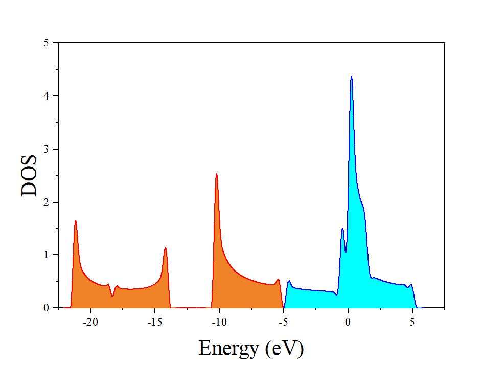
calculaiton='nscf'并增加kpoint的采样密度。cp -r scf dos cd dos mv scf.in nscf.in使用dos.x对nscf计算得态密度进行处理。输入文件
dos.in如下:&DOS prefix = 'carbyne' outdir = './outdir' bz_sum = "smearing" ngauss = 0 degauss = 2.0d-2 DeltaE = 0.01 fildos = 'carbyne.dos' /
对计算出来的态密度采用OriginPro进行作图,(采用较密kpoint计算的结果)如下所示。
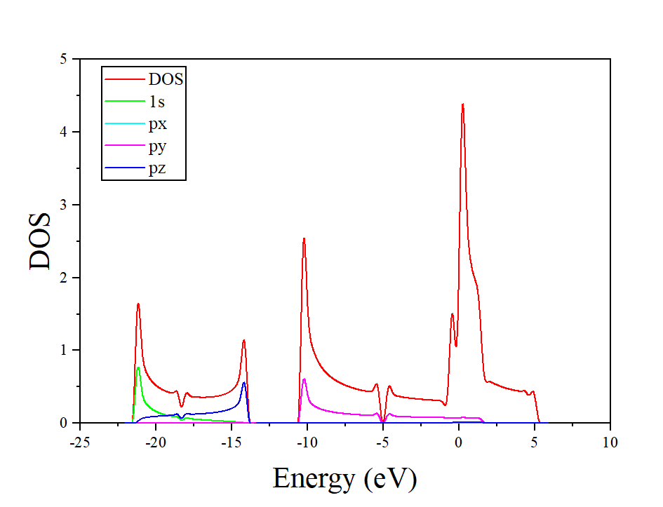
采用 projwfc.x 对态密度进行分波态密度计算,用于bandfat分析,后面进行Wannier计算,需要根据分波态密度来选取初始猜测的wannier函数。
projwfc.in

 &PROJWFC
prefix = 'carbyne'
outdir = './outdir'
ngauss = 0
degauss= 0.01
DeltaE = 0.5
filpdos= 'carbyne.pdos'
filproj= 'carbyne.proj'
/

projwfc.x <projwfc.in>projwfc.out
处理分波态密度得到的结果如下:
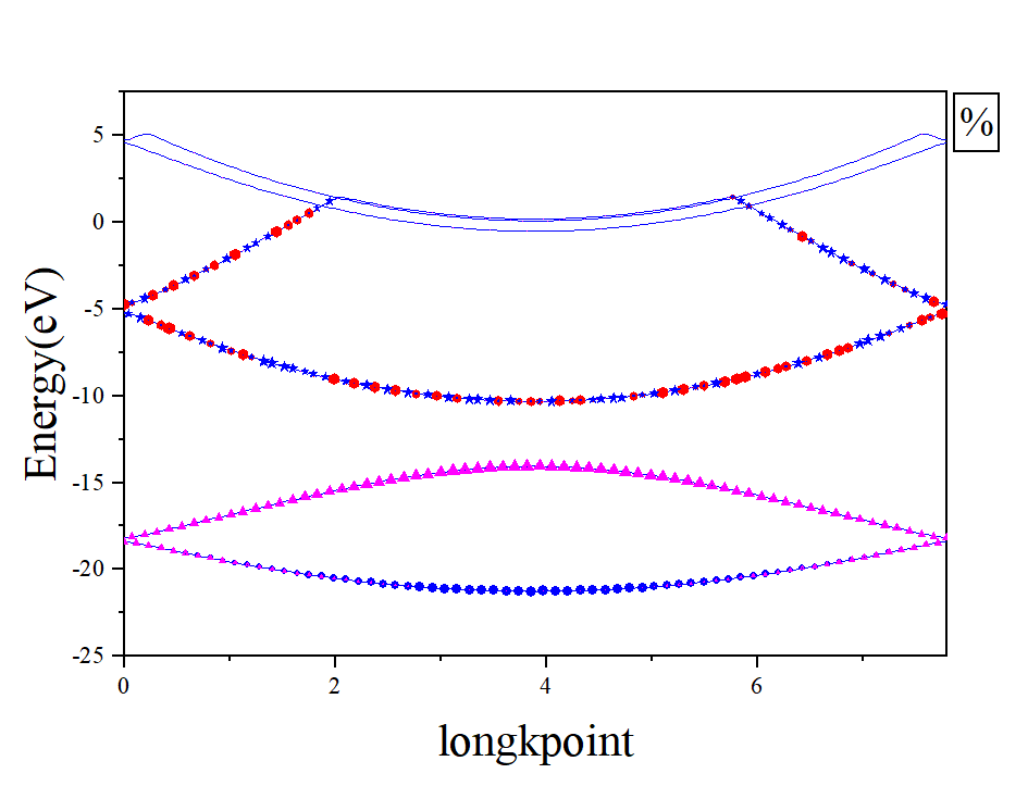
2.5 计算能带,修改
calculation='bands',nbnd和K_POINTS crystal_b部分进行第一布里渊区高对称kpoint的能带计算。cp -r scf band cd band cp scf.in pw-bands.in calculation = "bands" nbnd = 22 K_POINTS crystal_b 3 -0.5 0.0 0.0 50 0.0 0.0 0.0 50 0.5 0.0 0.0 1
计算完成后使用bands.x处理能带数据。在能带计算之后,用projwfc.x生成的fatband.projwfc_up文件,可以和bands.x生成的文件bands.dat结合,画出各个能带的原子轨道投影,画图脚本如下:/LVCSH/tools/fatband.f90。
计算能带图如下:
2.6 根据fatband中的结果,进行wannier90计算
2.6.1 Scf计算
2.6.2 nscf计算
cp scf.in nscf.in并做如下修改
calculation   = "nscf"
nbnd        = 16
!K_POINTS {automatic}
! 1  1  40  0 0 0

kmesh.pl 1 1 40 >>nscf.in
pw.x < nscf.in > nscf.out
2.6.3 Wannier90计算
!System
num_wann  = 4
num_bands = 6

!Projection
begin projections
C : px;py
end projections

!Job Control
exclude_bands : 1-2
!restart =

!disentanglement
dis_win_min  = -25.0
dis_win_max  = 7.0
dis_froz_min = -12.0
dis_froz_max = -0.6
dis_num_iter = 1000
dis_mix_ratio= 0.5
dis_conv_tol = 1.0E-10
dis_conv_window = 5

!Wannierise
num_iter = 10000
conv_tol = 1.0E-10
conv_window     = 10
guiding_centres = .true.

! SYSTEM

begin unit_cell_cart
Ang
  20.000000   0.000000   0.000000
  0.000000  20.000000   0.000000
  0.000000   0.000000   2.565985410
end unit_cell_cart

begin atoms_cart
Ang
C       10.0000000000       10.0000000000       -0.0019756118
C       10.0000000000       10.0000000000        1.2517014809
end atoms_cart

! KPOINTS
echo "mp_grid = 1 1 40">>${seedname}.win
echo "begin kpoints">>${seedname}.win
kmesh.pl 1 1 40 wannier >>${seedname}.win
echo "end kpoints">>${seedname}.win
2.6.4 'wannier90.x -pp seedname'
2.6.5pw2wannier90.x < pw2wan.in > pw2wan.outpw2wan.in &inputpp outdir = './outdir' prefix = 'carbyne' seedname = 'carbyne' spin_component = 'none' write_mmn = .true. write_amn = .true. write_unk = .true. /
2.6.6
mpirun -np $NP wannier90.x seedname通过wannier90计算,找到进行wannier拟合的相关参数设置,后续用于EPW计算中wannier拟合相关部分参数的设置。2.7 采用DFPT进行phonon计算。(为了后续数据处理,phonon计算需要设置的
outdir='./'),为了声子谱计算的更准确,scf计算中可以使用更密的K点,更少的q点。
2.7.1cp -r scf phonon, 设置scf.in 输入文件.其中电子自洽收敛需要设置的高一些,这样后续采用DFPT计算声子谱和电声耦合值会有更高精度。nbnd的设置对后续电声耦合计算无影响,K_POINTS的设置需要注意,后面EPW计算中需要与DFT计算的设置相同,K_POINTS的值可以设置的高一些,以使得phonon band计算出来的声子谱收敛。outdir = './' !nbnd = 22 conv_thr = 1.0e-9 K_POINTS {automatic} 40 1 1 0 0 0
2.7.2 进行phonon计算。
tr2_ph=1.0d-16需要设置的精度高一些。必须设置fildvscf以输出自洽势对normal mode的导数。phonons calculation &inputph ! recover = .true. tr2_ph = 1.0d-16, prefix = 'carbyne', outdir = './' lraman = .true. ! epsil = .true. !use for insulators ldisp = .true. nq1 = 40 nq2 = 1 nq3 = 1 ! amass(1) = 0.0 fildyn = 'carbyne.dyn' fildvscf = 'dvscf' /
2.7.3 采用q2r.x进行力常数矩阵的傅里叶变换,得到实空间中的动力学矩阵,并添加声学支求和,使得$\Gamma$点的声学支频率求和为0.
&input
fildyn='carbyne.dyn', zasr='simple', flfrc='flfrc'
/
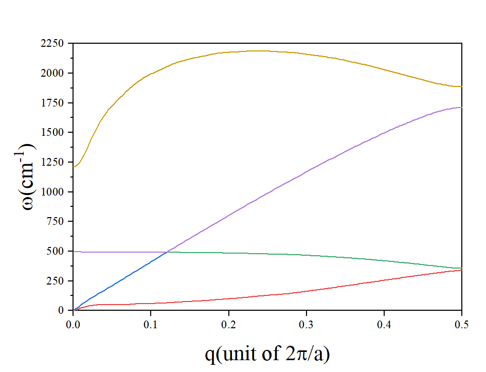
2.7.4 使用matdyn.x 对实空间中力常数矩阵进行逆傅里叶变换,计算声子谱和声子态密度。
&input
asr='simple',
!amass(1)=26.98, amass(2)=74.922,
flfrc='flfrc',
flfrq='phonon-freq',
q_in_band_form=.true.,
/
2
0.0 0.0 0.0 100
0.5 0.0 0.0 1
使用plotband.x处理声子谱数据。plotband.in
phonon-freq
0 4000
phonon-freq.plot
phonon-freq.ps
0.0
0.1 0.0
计算得到的声子谱如下图所示:
2.7.5 使用matdyn.x计算声子态密度. matdyn-dos.in
&input
    asr='simple',
!   amass(1)=26.98, amass(2)=74.922,
    flfrc='flfrc',
!    flfrq='flfrq',
!    la2F=.true.
    dos=.true.
    fldos="phonon-dos"
    nk1=1,nk2=1,nk3=100
/
2.7.6 使用pp.py(位于目录EPW/bin下)收集ph.x计算得到的fildvscf相关文件到save文件夹。
2.8 EPW 计算电声耦合强度.计算电声耦合强度需要在scf计算和phonon计算中采用较高的收敛判据。包括:
etot_conv_thr,forc_conv_thr,press_conv_thr,conv_thr,tr2_ph-
第一步:进入phonon目录进行scf自洽计算
-
第二步:ph.x进行DFPT计算(最费时间,需要注意设置参数
fildyn和fildvscf)
在phonon计算中可以使用-nimage N参数进行并行计算,可以在不同的节点上计算不同的q点。On parallel machines the q point and the irreps calculations can be split automatically using the -nimage flag. See the phonon user guide for further information.mpirun -np $NP -machinefile ${CURDIR}/nodelist ph.x -ni 6 -npool 28 <ph.in> ph.out`
-
第三步:使用pp.py收集ph.x计算得到的fildvscf相关文件到save文件夹
-
第四步:进入epw目录,先进行scf计算(或者将phonon目录中的内容拷贝过来),再进行nscf计算,需要设置所有的k点并且修改
nbnd的值。scf计算和nscf计算需要使用与phonon计算时相同的参数设置和计算精度。
kmesh.pl 40 1 1 >>${prefix}.nscf.in -
第五步,设置 epw.in 文件,进行epw计算,设置
prtgkk以及ephwrite.注意fsthick的设置,会影响打印出来的电声耦合矩阵元包含的能带数和q点数。EPW计算完成后需要检查插值后的phonon的频率(插值可能导致出现虚频,与wannier插值傅里叶变换有关,可能需要重新设置wannier插值参数)。epw.in如下:
epw calculation of carbyne &inputepw prefix = 'carbyne' outdir = './' amass(1)= 12.0107 dvscf_dir = '../phonon/save/' iverbosity = 0 elph = .true. ep_coupling = .true. ! epbwrite = .true. ! epbread = .false. epwwrite = .true. epwread = .false. ! etf_mem = 1 prtgkk = .true. ! ephwrite = .true. ! eig_read = .true. lifc = .true. asr_typ = 'crystal' wannierize = .true. nbndsub = 4 bands_skipped = 'exclude_bands = 1-2' num_iter = 10000 iprint = 2 ! dis_win_max = 12 ! dis_win_min = -25 ! dis_froz_min = -11 dis_froz_max = -0.2 proj(1) = 'C:py;pz' ! proj(2) = 'C:sp-1' write_wfn= .true. wannier_plot= .true. wdata(1)= 'bands_plot = .true.' wdata(2)= 'begin kpoint_path' wdata(3)= 'G 0.00 0.00 0.00 M 0.50 0.00 0.00' wdata(4)= 'end kpoint_path' wdata(5)= 'bands_plot_format = gnuplot' wdata(6)= 'conv_tol = 1.0e-10 ' wdata(7)= 'conv_window = 3 ' wdata(8)= 'dis_conv_tol = 1.0e-10 ' wdata(9)= 'dis_conv_window = 3 ' wdata(10)= 'dis_num_iter= 10000 ' wdata(11)= 'dis_mix_ratio= 0.5 ' wdata(12)= 'guiding_centres = .true.' wdata(13)= 'translate_home_cell : true' wdata(14)= 'translation_centre_frac : 0.0 0.0 0.0 ' elecselfen = .false. phonselfen = .false. a2f = .false. fsthick = 5.0 ! eV temps = 1 ! K degaussw = 0.005 ! eV nkf1 = 40 nkf2 = 1 nkf3 = 1 nqf1 = 40 nqf2 = 1 nqf3 = 1 nk1 = 40 nk2 = 1 nk3 = 1 nq1 = 40 nq2 = 1 nq3 = 1 /-
EPW声子谱和QE不一致 (参考简书)
这个问题一般是由于声子求和规则导致的,EPW中提供了读入实空间力常数来计算声子频率的方法,并且也提供了相应的声子求和规则(与matdyn.f90里面的相同)。只需要改lifc = .true.,然后再设置声子求和规则asr_typ = crystal(我一般都取crystal),同时需要注意的是要保证之前计算QE得到的文件通过pp.py收集起来那个必须有q2r.x产生的实空间力常数文件并且已经被命名为 ifc.q2r,对于包含SOC的情况,这个文件必须叫 ifc.q2r.xml 并且是xml格式的文件。(这个一般不是太老的脚本pp.py都会自动帮你做这件事情。)参考phonon bandstructure from EPW and matdyn.x don't match&input fildyn='carbyne.dyn', zasr='simple', flfrc='ifc.q2r' /
-
第六步,使用第五步
epwwrite=.true.设置输出的wannier表象下的电声耦合文件,计算不同nqf和nkf插值密度的EPW计算。使用runepw.sh脚本进行提交计算:
#!/bin/bash
for i in $(seq 20 20 240)
        do
        cp epw.in epw${i}.in
        sed -i "s:epwwrite:epwwrite=.false. ! :g" epw${i}.in
        sed -i "s:epwread:epwread=.true. !:g" epw${i}.in
        sed -i "s:prtgkk:prtgkk=.true. !:g" epw${i}.in
        sed -i "s:wannierize:wannierize=.false. !:g" epw${i}.in
        sed -i "s:nkf1:nkf1=$i !:g" epw${i}.in
        sed -i "s:nqf1:nqf1=$i !:g" epw${i}.in

        cp qe-epw.bsub qe-epw${i}.bsub
        sed -i "2s:epw:epw${i}:g" qe-epw${i}.bsub
        sed -i "s:epw.in:epw${i}.in:g" qe-epw${i}.bsub
        sed -i "s:epw.out:epw${i}.out:g" qe-epw${i}.bsub

        bsub < qe-epw${i}.bsub
        sleep 10
        done
- 上述脚本,有可能由于epwread文件读取冲突,导致不能正常计算,使用下列命令,找出不能正常running的作业,重新提交。
for i in $(seq 20 20 240);do echo epw$i.out;head epw$i.out;done
- In directory epw to calculate the electron-phonon coupling matrix using the changed EPW code. And the output be named dependend on the kpoint: as epw40.out, epw80.out, epw120.out, epw160.out. Used to test the kpoint and qpoint convergence.
-
-
构建目录,进行LVCSH.x的串行计算(只能单核计算,程序内的并行计算待开发),需要测试
lit_ephonon的值,由于低频声学支声子部分可能会导致计算结果发散,(低频声学支会导致Normal mode极大)mkdir LVCSH-epw40 cp ./epw/epw40.out ./LVCSH-epw40 cd LVCSH-epw40 vi LVCSH.in LVCSH_complex.x &
calculation   = "lvcsh" ! "lvcsh" or "plot"
verbosity     = "low"   ! "low" or "high"
l_dEa_dQ      = .false.
l_dEa2_dQ2    = .false.
outdir        = "./"
methodsh      = "FSSH"
lit_gmnvkq    = 0.0    ! in unit of meV
lit_ephonon   = 0.0    ! in unit of meV
eps_acustic   = 5.0    ! in unit of cm-1
lfeedback     = .true.
lehpairsh     = .true.
!lelecsh       = .true.
!lholesh       = .true.
!ieband_min    = 3
!ieband_max    = 4
!ihband_min    = 1
!ihband_max    = 2
!lsortpes      = .false.
!mix_thr       = 0.8
epwoutname    = "./epw.out"
!nefre_sh      = 40
!nhfre_sh      = 40
nnode         = 1
ncore         = 1
naver         = 2000
nsnap         = 1000
nstep         = 2
dt            = 0.5
savedsnap     = 25
ldecoherence  = .true.
Cdecoherence  = 0.1
l_ph_quantum  = .true.
temp          = 300
pre_nstep     = 50000
pre_dt        = 0.5
!gamma         = 0.0   ! in unit of ps-1
ld_fric       = 0.01   !
llaser        = .true.
efield_cart   = 1.0 1.0 1.0
w_laser       = 2.0  ! in unit of eV
fwhm          = 100  ! in unit of fs
-
构建目录使用手动方式进行LVCSH.x的并行计算(在不同的节点和核上进行不同轨迹的计算,计算完成后使用LVCSH.x程序后处理取平均值.)
make a directory LVCSH for lvcsh calculation。并在LVCSH目录下放入LVCSH.in输入文件,以及并行计算的脚本和任务提交脚本bsub脚本。mkdir LVCSH
3.1 make a lsf job script. Need to change the BUSB -q,-n,-R and MODULEPATH as your Environment.
lvcsh.bsub
#!/bin/bash
#BSUB -J JOB_NAME
#BSUB -q QUEUE_NAME
#BSUB -n ncore
#BSUB -R "span[ptile=ncore]"
#BSUB -o %J.out
#BSUB -e %J.err

#source ~/xh/.bashrc
#export OMP_NUM_THREADS=1
#export MKL_NUM_THREADS=1
export MODULEPATH=$MODULEPATH:DIR_MODULEPATH

module load lvcsh/version

CURDIR=$PWD
#Generate nodelist
rm -f ${CURDIR}/nodelist >& /dev/null
for i in `echo $LSB_HOSTS`
do
echo $i >> ${CURDIR}/nodelist
done

NP=`cat ${CURDIR}/nodelist |wc -l`

for i in $(seq 1 1 $NP)
do
mkdir sample$i
cp ./LVCSH.in ./sample$i/
cd ./sample$i
LVCSH_complex.x &
cd ..
done
wait
3.2 Use shell script mkepwdir.sh to build dir for diffrent kpoints and qpoints Surface hopping calculation. And the script will make a test running in the different director to give how to set
nefre_shandnhfre_sh.mkepwdir.sh #!/bin/bash ncore=28 MODULEPATH="/share/home/zw/xiehua/opt/modules-4.7.1/modulefiles" lvcsh_version="0.6.6" QUEUE_NAME="privateq-zw" for i in $(seq 80 40 80) do mkdir epw$i mkdir epw$i/QEfiles cp ../epw/epw$i.out epw$i/QEfiles/ cp lvcsh.bsub epw$i sed -i "s/ncore/$ncore/g" epw$i/lvcsh.bsub sed -i "s:JOB_NAME:lvcsh-epw${i}-n0:g" epw$i/lvcsh.bsub sed -i "s:QUEUE_NAME:$QUEUE_NAME:g" epw$i/lvcsh.bsub sed -i "s:DIR_MODULEPATH:$MODULEPATH:g" epw$i/lvcsh.bsub sed -i "s:version:$lvcsh_version:g" epw$i/lvcsh.bsub cp job.sh epw$i cp LVCSH.in epw$i sed -i "s:./epw.out:../../QEfiles/epw$i.out:g" epw$i/LVCSH.in sed -i "s:ncore:ncore = $ncore !:g" epw$i/LVCSH.in cp lvcsh-test.bsub epw$i/lvcsh-plot.bsub sed -i "2s/JOB_NAME/lvcsh-epw$i-plot/g" epw$i/lvcsh-plot.bsub sed -i "s:QUEUE_NAME:$QUEUE_NAME:g" epw$i/lvcsh-plot.bsub sed -i "s:DIR_MODULEPATH:$MODULEPATH :g" epw$i/lvcsh-plot.bsub sed -i "s:version:$lvcsh_version:g" epw$i/lvcsh-plot.bsub cp LVCSH.in epw$i/QEfiles sed -i "s:verbosity:verbosity = "high" !:g" epw$i/QEfiles/LVCSH.in sed -i "s:./epw.out:./epw$i.out:g" epw$i/QEfiles/LVCSH.in sed -i "s:naver:naver = 10 !:g" epw$i/QEfiles/LVCSH.in sed -i "s:nsnap:nsnap = 2 !:g" epw$i/QEfiles/LVCSH.in sed -i "s:savedsnap:savedsnap = 2 !:g" epw$i/QEfiles/LVCSH.in cp lvcsh-test.bsub epw$i/QEfiles cd epw$i/QEfiles sed -i "2s/JOB_NAME/lvcsh-epw$i-test/g" lvcsh-test.bsub sed -i "s:QUEUE_NAME:$QUEUE_NAME:g" lvcsh-test.bsub sed -i "s:DIR_MODULEPATH:$MODULEPATH :g" lvcsh-test.bsub sed -i "s:version:$lvcsh_version:g" lvcsh-test.bsub bsub < lvcsh-test.bsub cd ../.. done
job.sh
#!/bin/bash
    nnode=10
    sed -i "s:nnode:nnode         = $nnode !:g" LVCSH.in
    for i in $(seq 1 1 $nnode)
    do
    mkdir node$i
    cp ./lvcsh.bsub ./node$i/
    sed -i "2s/n0/n$i/g" ./node$i/lvcsh.bsub
    cp ./LVCSH.in ./node$i/
    cd ./node$i
    bsub < lvcsh.bsub
    cd ..
    done
LVCSH.in
calculation   = "lvcsh" ! "lvcsh" or "plot"
verbosity     = "low"   ! "low" or "high"
l_dEa_dQ      = .false.
l_dEa2_dQ2    = .false.
outdir        = "./"
methodsh      = "FSSH"
lit_gmnvkq    = 0.0    ! in unit of meV
lit_ephonon   = 0.0    ! in unit of meV
eps_acustic   = 5.0    ! in unit of cm-1
lfeedback     = .true.
lehpairsh     = .true.
!lelecsh       = .true.
!lholesh       = .true.
ieband_min    = 9
ieband_max    = 9
ihband_min    = 8
ihband_max    = 8
!lsortpes      = .false.
!mix_thr       = 0.8
epwoutname    = "./epw.out"
!nefre_sh      = 40
!nhfre_sh      = 40
nnode         = 1
ncore         = 1
naver         = 5000
nsnap         = 1000
nstep         = 2
dt            = 0.5
savedsnap     = 25
ldecoherence  = .true.
Cdecoherence  = 0.1
l_ph_quantum  = .true.
temp          = 300
pre_nstep     = 5000
pre_dt        = 0.5
!gamma         = 0.0   ! in unit of ps-1
ld_fric       = 0.01   !
llaser        = .true.
efield_cart   = 1.0 1.0 1.0
w_laser       = 2.0  ! in unit of eV
fwhm          = 100  ! in unit of fs
lvcsh-test.bsub
#!/bin/bash
#BSUB -J JOB_NAME
#BSUB -q QUEUE_NAME
#BSUB -n 1
#BSUB -o %J.out
#BSUB -e %J.err

export MODULEPATH=$MODULEPATH:DIR_MODULEPATH

module load lvcsh/version

LVCSH_complex.x
3.3 By look the initial adiabatic state in the QEfiles/LVCSH.out for different kpoints directory. Set the
nefre_shandnhfre_shin the QEfiles/LVCSH.in to tests the time for one step nonadiabatic calculation. Then, subscrib the job again.bsub < lvcsh-test.bsub3.4. change the LVCSH.in file in the epw40, including the parameters for lvcsh run as following:
ieband_min    = 9
ieband_max    = 9
ihband_min    = 8
ihband_max    = 8
epwoutname    = "../../QEfiles/epw120.out"
nefre_sh = 34
nhfre_sh = 34
nnode    = 10
ncore    = 28
naver    = 100
nstep    = 2
nsnap    = 1000
dt       = 0.5
savedsnap= 25
change the
nnodesin the job.sh bash script. Then './job.sh' to make lvcsh running innnodesnode, which includencoreCPU cores.3.5 After the setp 7, change the parameter
calculation = plotandepwoutname = './QEfiles/epw40.out'of LVCSH.in in the direpw40. Then runLVCSH_complex.xinepw40dir. The code will read the result in all nodes and cores, then get a average results and writing in the direpw40.