Drone-enabled forest ecology: A fine-grain, broad-extent analysis of how forest structure and regional climate interact to influence the western pine beetle-induced mortality rate of ponderosa pine in the Sierra Nevada Mountain range of California during the exceptional hot drought of 2012-2015.
The manuscript describing this work was published in Nature Communications in 2021:
Koontz, M.J., Latimer, A.M., Mortenson, L.A. et al. Cross-scale interaction of host tree size and climatic water deficit governs bark beetle-induced tree mortality. Nat Commun 12, 129 (2021). https://doi.org/10.1038/s41467-020-20455-y
This repository represents the workflow used to process the drone data from aerial photographs taken over ~40 ha of forested area surrounding each of 32 field plots along a 350 km latitudinal gradient and 1,000 m elevational gradient on the western slope Sierra Nevada in yellow pine/mixed-conifer forests. In total, over 9 km^2^ of forest was surveyed between early April, 2018 and early July, 2018 at a spatial resolution of approximately 8 cm per pixel. The coincident field sites (described in Fettig et al., 2019) were selected to have >40% ponderosa pine tree by basal area and >10% mortality of ponderosa pine tree by basal area.
Over 450,000 photographs were captured for this study: approximately 75,000 were captured using a broad band RGB camera, and approximately 75,000 were captured using a Micasense RedEdge narrow band multispectral camera with 5 discrete bands of sensitivity (blue, green, red, red edge, and near infrared). Each image capture with the Micasense RedEdge camera resulted in 5 images generated, one for each narrow band (for a total of 375,000 photographs).
The workflow is detailed in the workflow/ directory, and the files are numbered with the order in which they were run. Data related to the drone-acquired imagery are organized using "data product levels" akin to those used by NASA and USGS and are located in the data/data_drone/ directory under their appropriate Level subdirectory (L0, L1, L2, L3a, L3b, L4). In a general sense, Level 0 data represent raw data from the instruments (original photographs and flight logs) while each higher level represents data derived from levels below it. See Figure 2 in the manuscript as well as the methods section for more details on this file organization structure.
Level 0 data occupy approximately 1.2 TB of disk space. Level 1 data occupy approximately 49.1 GB of disk space. Level 2 data occupy approximately 71.1 GB of disk space. Level 3a data occupy approximately 1.7 GB of disk space. Level 3b data occupy approximately 3.7 GB of disk space. Level 4 data occupy approximately 46.9 MB of disk space.
Due to the high volume of data processing required for the project, the Structure from Motion photogrammetry step was performed in a separate directory (data/data_working/) from the final home of the drone-related data (data/data_drone/). The software used for the Structure from Motion photogrammetry, Pix4Dmapper, creates a lot of additional files and a very complicated file structure, so some of the workflow files copy and rename files from the default Pix4D output and save them instead in a consistent and more readily discoverable part of the data/data_drone/ directory (e.g., workflow/15_rehome-pix4d-report-dsm-dense-point-cloud.R).
Script files labeled with an 'x' after their number represent workflow steps that were specific to this paper and are not expected to be part of a general drone forest ecology workflow (e.g., estimating geolocation for some Micasense RedEdge photographs using known geolocations from the co-mounted RGB camera, then writing that information to the RedEdge photographs' EXIF metadata to aid the Structure from Motion process). The number in these files still represents the order in which these idiosyncratic workflow steps were run. In one case, workflow/06x_alternative_rename-and-integrate-x3-and-re-photos.R), the script should be run in place of the script with the similar name (workflow/06_rename-and-integrate-x3-and-re-photos.R). In all other 'x' cases, the script is run in addition to the other scripts in the workflow.
The file organization for the drone-related data looks like this:
local-structure-wpb-severity
|--analyses/
|--docs/
|--figures/
|--workflow/
|__data/
   |--data_raw/
   |--data_output/
   |__data_drone/
      |--L0/
      |  |--flight-logs/
      |  |--photos/
      |  |--photos-metadata/
      |  |--mission-footprint/
      |  |  |--photo-points/
      |  |  |--site-bounds/
      |  |  |__srtm30m/
      |  |__surveyed-area-3310.gpkg
      |
      |--L1/
      |  |--pix4d-reports/
      |  |--plot-locations/
      |  |--ortho/
      |  |--dsm/
      |  |--dense-point-cloud/
      |  |--ground-trees.gpkg
      |  |__plot-centers-identifiable-from-air_3310.gpkg
      |
      |--L2/
      |  |--index/
      |  |--classified-point-cloud/
      |  |--dtm/
      |  |__chm/
      |
      |--L3a/
      |  |--ttops/
      |  |__crowns
      |
      |--L3b/
      |  |--hand-classified-trees/
      |  |--model-classified-trees/
      |  |--crowns-with-reflectance/
      |  |--crowns-with-reflectance_all.csv
      |  |--crowns-with-reflectance_35m-buffer.csv
      |  |--hand-classified-trees_all.csv
      |  |__model-classified-trees_all.gpkg
      |
      |__L4/
         |--rasterized-trees/
         |__data-from-rasterized-classified-trees.csv
The general workflow is:
- Fly a grid pattern over a forested site using a DJI drone and the Map Pilot for iOS iPad app.
- Take images every 2 seconds during the flight with lots of overlap between images.
- Use photogrammetry (a.k.a. "structure from motion") software to turn the overlapping 2D images into a 3D point cloud, a 2D surface model, and a 2D orthomosaic. We use the Pix4D software and adjust processing parameters to best account for dense vegetation.
- Use a point cloud manipulation software to classify the 3D point cloud into "ground" and "non-ground" points using a "cloth simulator filter". This filter also has the effect of using the classified "ground" points to generate a 2D continuous digital terrain model underneath the vegetation. We use CloudCompare for this.
- Generate a "canopy height model" by subtracting away the CloudCompare generated terrain model from the Pix4D generated 2D surface model to leave just the surface representing the vegetation.
- We use a variable window local maximum filter to identify the tree tops in the canopy height model. (In
Rusing theForestToolspackage) - We use a marker controlled watershed segmentation algorithm to identify the pixels in the orthomosaic that are associated with the individual trees. (Also in
Rand using theForestToolspackage) - We extract the red, blue, and green values from the pixels of the orthomosaic representing each tree. We calculate the red-green index (RGI) as R / G and the red-green vegetation index as (R - G) / (R + G). We take the average and the 75th percentile of these 5 metrics across all pixels belonging to each tree.
- Using QGIS, we overlay the polygons of the segmented crowns on top of the the RGB orthomosaic for the eldo_3k_1, eldo_5k_1, sequ_4k_1, and sequ_6k_1 sites. We made a copy of the segmented crowns polygons and added an attribute field called "live". We then panned around the orthomosaic and manually changed the "live" field for ~100 trees per site to 0 (for a dead tree) or 1 (for a live tree).
- Using the ~400 manually classified crown segments and the orthomosaic for each site, we extract the R, G, B, RGI (RGI = R/G per pixel), and GBI (GBI = G/B per pixel) data from each pixel and take the mean value of each spectral signature across all the pixels within each crown polygon. Using the mean R, G, B, RGI, and GBI values per crown polygon as covariates, We fit a generalized linear model using a binomial family and a logit link to predict the probability that the tree represented by the crown segment was alive or dead.
- Next, we extracted the R, G, B, RGI, and GBI means for all the crown polygons from each site's orthomosaic. We used the
veloxpackage inRto do this massive pixel value extraction from the raster files. - We used the logistic regression model that we fit above to predict the probability that each tree in the study (across all sites) was alive or dead.
Some photos of the processing:
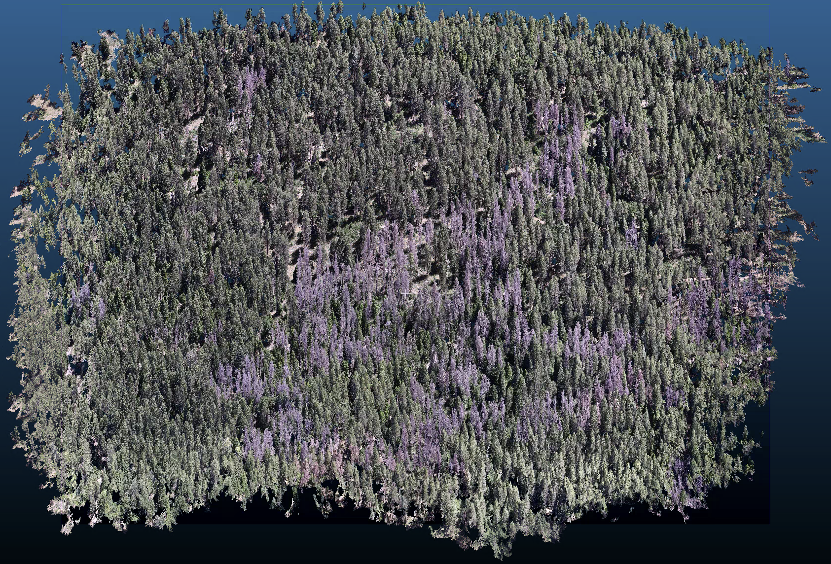
This is one of the data products from the Pix4D processing of the 2D aerial imagery. Here, the point cloud is visualized using the CloudCompare software.
This is a portion of one of the other primary data products of the Pix4D processing-- an orthomosaic showing the top-down view of all objects in the scene with the spatial relationships amongst them preserved. This image is suitable for making measurments between the trees.
This is a view of just the points from the point cloud classified as "ground" after using the cloth simulator function in CloudCompare. Essentially, the trees from the previous image have been "deleted" off the landscape.
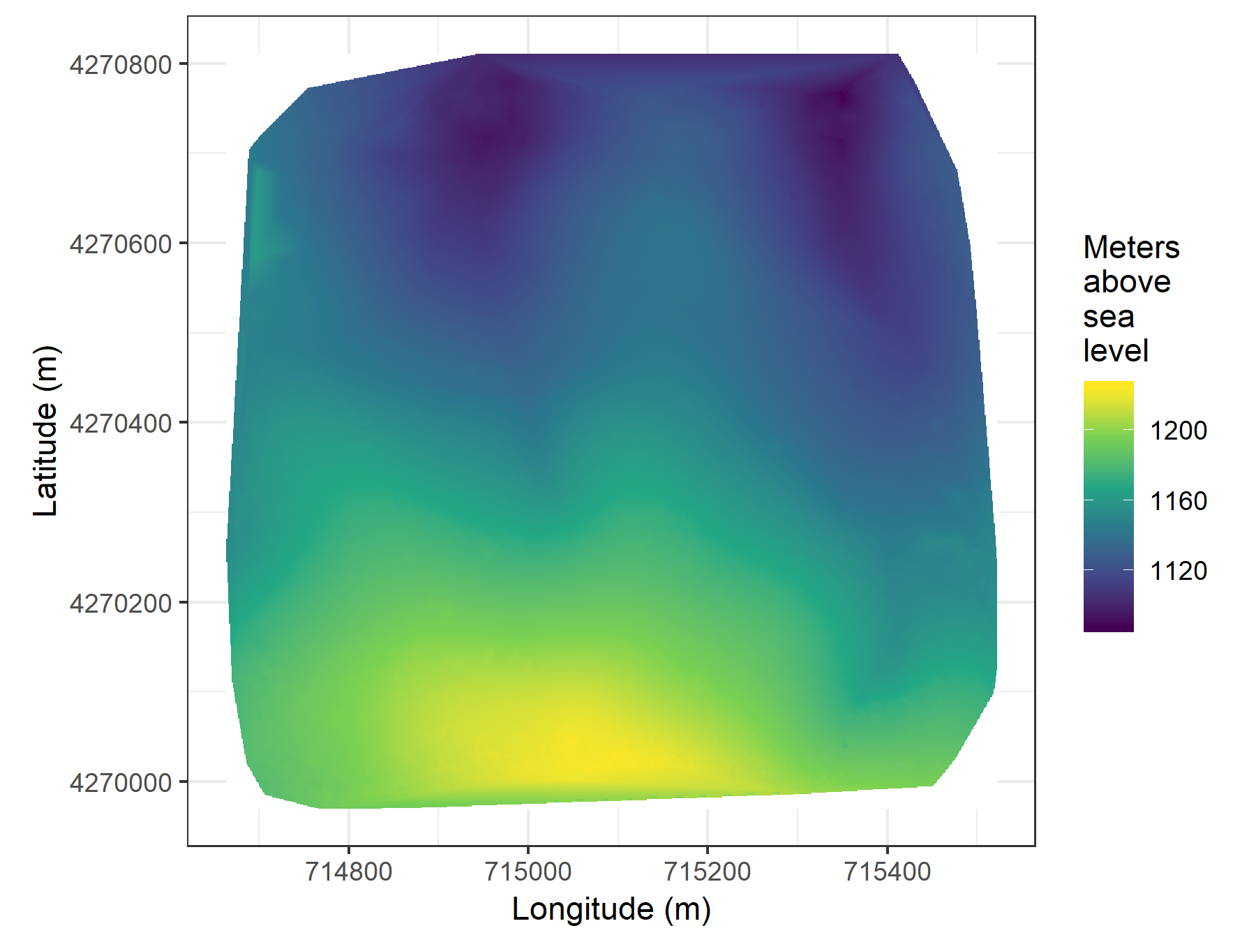
We can use the same "cloth" that helped classify ground versus non ground to interpolate the terrain underneath the trees, even where the trees may have obscured the ground. In 2 dimensions, the digital terrain model looks like this:
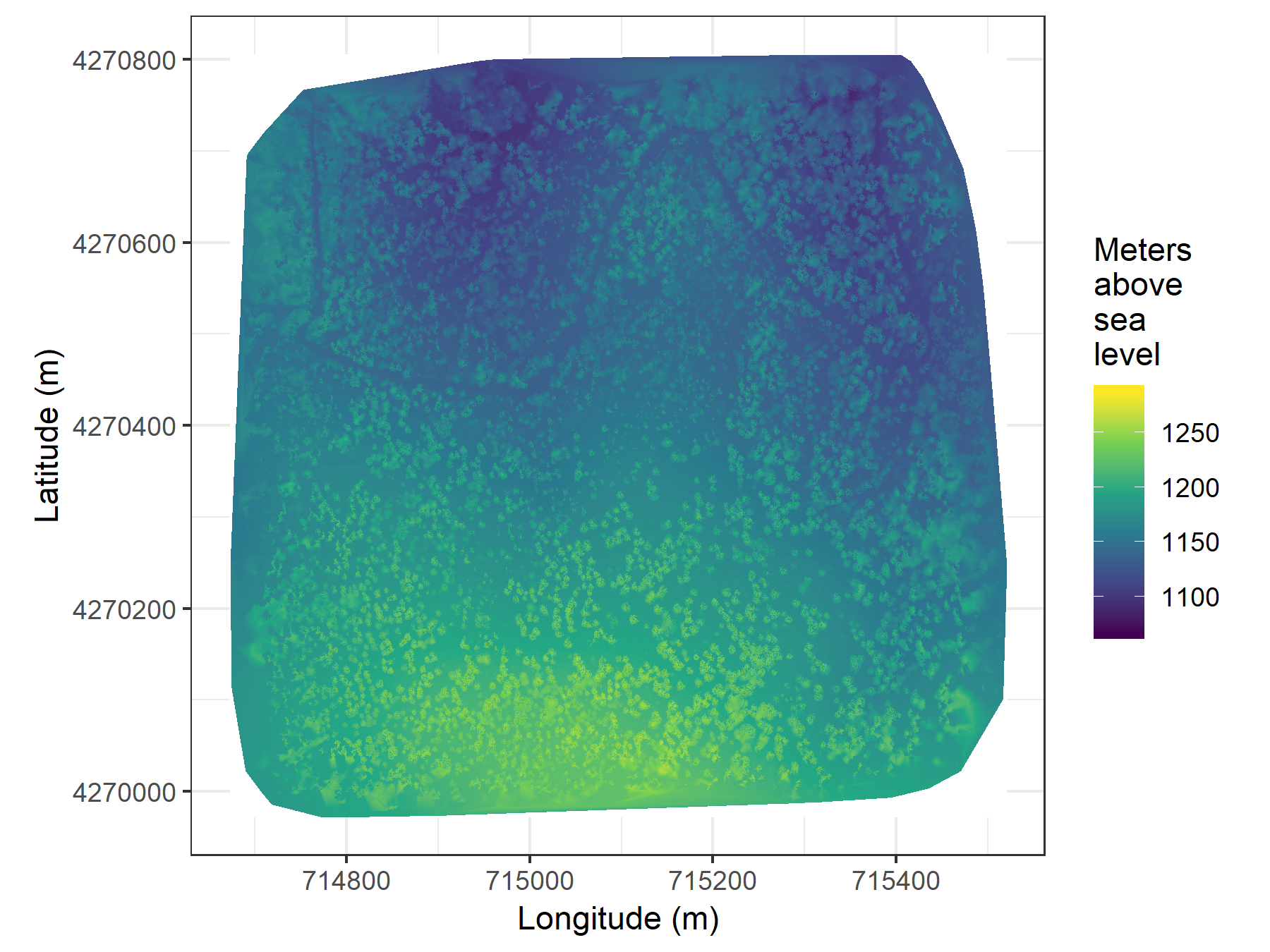
The Digital Surface Model is an output from Pix4D that represents the height of the surface, which includes the elevation of the ground plus the height of the vegetation.
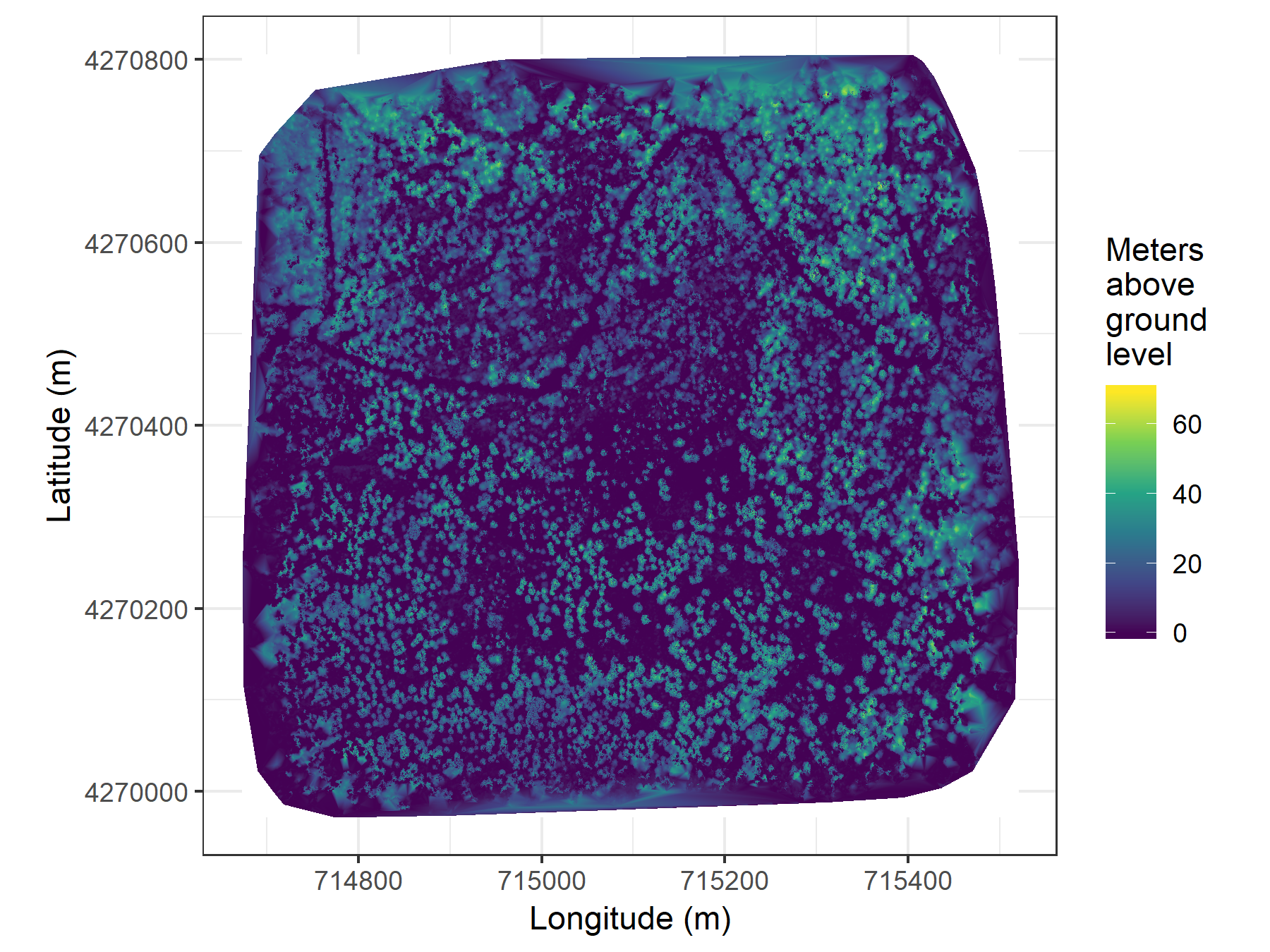
By subtracting the Digital Terrain Model (DTM) away from the Digital Surface Model (DSM), we get a representation of the heights of all the vegetation-- a Canopy Height Model (CHM).
The "variable window filter" algorithm detects tree tops as local maxima using the Canopy Height Model.
The tree top locations and the Canopy Height Model are then used to determine the spatial extent of each tree's crown using a marker controlled watershed segmentation algorithm.
The classification of all trees in the study (whether they were alive or dead) based on the extracted pixel values from the orthomosaic for each crown segment generates a "forest stem map" for each site.
We can use a different model to classify the live trees to species.


