microly / ggpolar

A ggplot2 Extension to Plot Data in Polar Coordinates on a Cartesian Layer

ggpolar

ggpolar supplies a few ggplot2 facilities to plot data in polar coordinates on a cartesian layer.

Highlights

• You can plot radius and theta on a cartesian layer directly, and draw the polar coordinates based plots intuitively.
• You can translate and/or rotate the data (even data in cartesian coordinates!) and/or the whole layer.
• ggpolar can interpolate data automatically, so you are able to draw arcs and sectors as easily as draw lines and polygons.
• ggpolar would not supply many layer functions, it tries to modify the layers! So you can plot and handle data in polar coordinates on the layers in ggplot2 package and its extension packages.

Installation

By now, ggpolar has not been submitted to CRAN. You can try the development version from GitHub:

# install.packages("devtools")
devtools::install_github("microly/ggpolar")

Usage

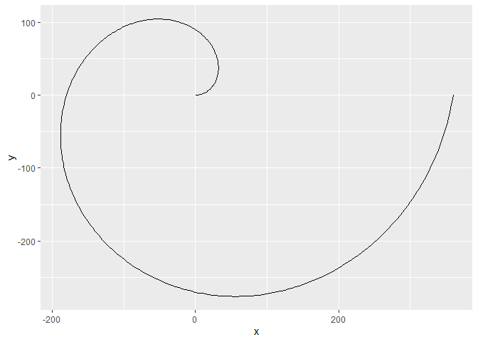
1.You can plot radius and theta to a layer directly.

library(tibble)
library(ggplot2)
library(ggpolar)

polar_data <- tibble(theta = 1:360, radius = theta)

# use StatPolar
ggplot(polar_data) + 
    geom_path(aes(p_theta = theta, p_radius = radius), stat = "polar")

# use with_polar, which is a layer modifier
ggplot(polar_data) + 
    with_polar(geom_path(aes(p_theta = theta, p_radius = radius)))
#> Warning: Ignoring unknown aesthetics: p_theta, p_radius

# the way to suppress the warning "Ignoring unknown aesthetics: p_theta, p_radius":
ggplot(polar_data, aes(p_theta = theta, p_radius = radius)) + 
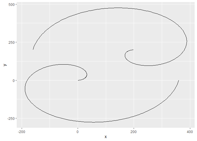
    with_polar(geom_path())

2.You can translate and/or rotate the data.

ggplot(polar_data, aes(p_theta = theta, p_radius = radius)) + 
    with_polar(geom_path(),
               geom_path(aes(translate_x = 200, translate_y = 200, rotate = 180)))
#> Warning: Ignoring unknown aesthetics: translate_x, translate_y, rotate

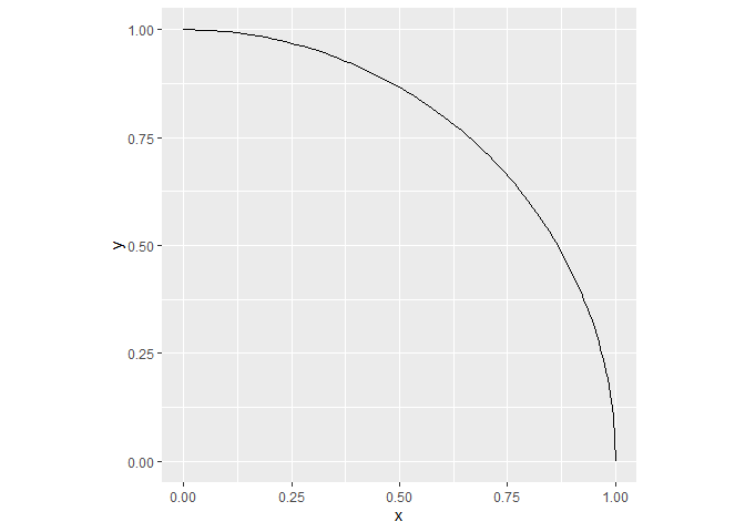
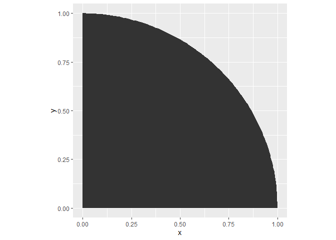
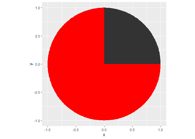
3.Data can be interpolated automatically, so you can draw arcs and sectors as easily as draw lines and polygons.

# you define the start and end points
polar_data2 <- tibble(theta = c(0,90), radius = 1)

# ggpolar will automatically interpolate other points.

# an arc example
ggplot(polar_data2, aes(p_theta = theta, p_radius = radius)) + 
    with_polar(geom_path(), interpolate = TRUE) + 
    coord_equal()

# a sector example
ggplot(polar_data2, aes(p_theta = theta, p_radius = radius)) + 
    with_polar(geom_polygon(), interpolate = TRUE, add_origin = TRUE) + 
    coord_equal()

# ggpolar can even make the supplement geometry for you! 
ggplot(polar_data2, aes(p_theta = theta, p_radius = radius)) + 
    with_polar(geom_polygon(), interpolate = TRUE, add_origin = TRUE) +
    with_polar(geom_polygon(fill = "red"), interpolate = TRUE, 
               supplement = TRUE, add_origin = TRUE) +
    coord_equal()

4.With the help of some layer functions (geom_plar_axis, geom_polar_ring and geom_polar_bar), you can draw the polar coordinates based plots (eg. radar plot, pie chart and Nightingale rose diagram) in a more intuitively way.

# I will add some examples later.