![]()

This library is still under active development and is not yet producing stable results. Use at your own risk.
OD-Toolbelt is a suite of tools for use with image object detection models.
OD-Toolbelt takes raw bounding box predictions from the object detection model of your choosing, post-processes them, and returns enhanced and filtered predictions. Think of it as a post-processing step you can add onto your object detection workflow to boost performance.
Modules:
- Suppressors: Different non-maximum suppression methodologies to select from.
- Selectors: A modular way to create selection logic for image suppression. See base/od_toolbelt/nms/selectors/README.md for more information on available selectors.
- Metrics: A modular way to create measures of bounding box overlap. See base/od_toolbelt/nms/metrics/README.md for more information on available metrics.
- ASAP-NMS (arXiv:2007.09785v2 [cs.CV])
In object detection machine learning models, typically several sets of overlapping bounding boxes are predicted for each given object in the image. Only a fraction of these bounding boxes are valid, and the others must be removed from the final prediction.
Given the following photo...
Feb 19, 2015 - morning sunrise, 02 by Ed Yourdon is licensed under CC BY-NC-SA 2.0

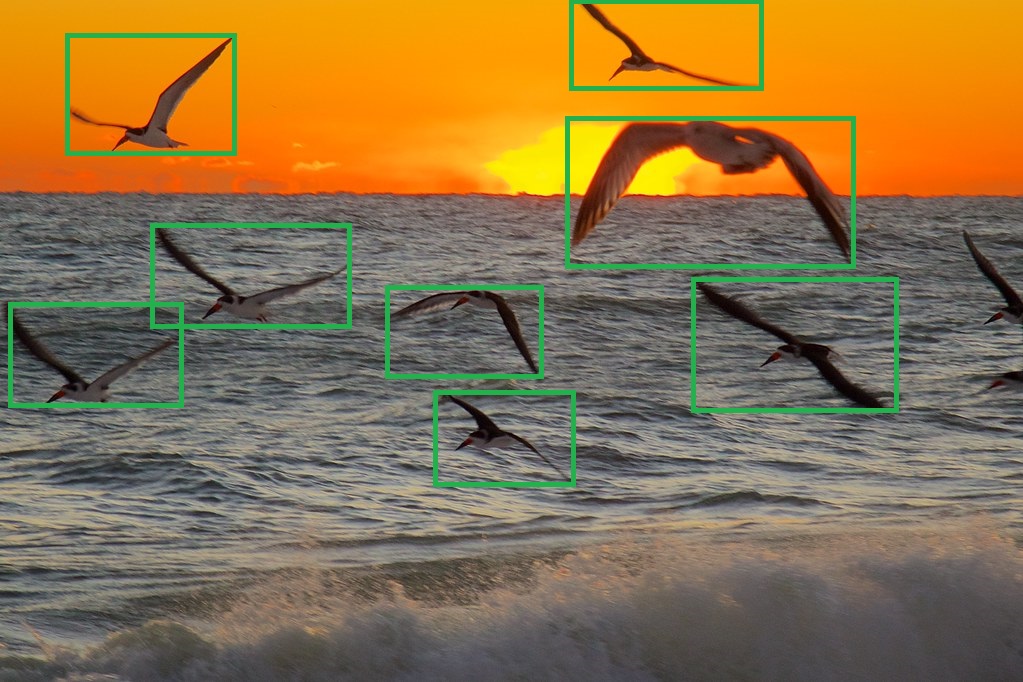
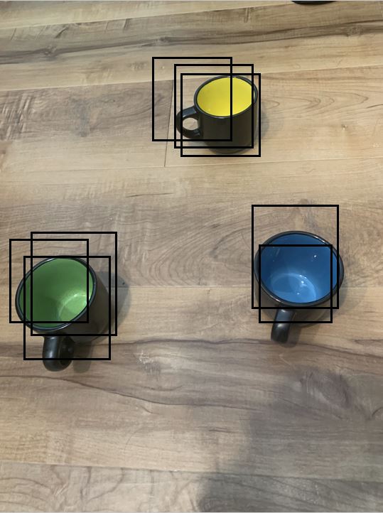
... we would normally expect the following predictions from an object detector trained to
detect birds.
Feb 19, 2015 - morning sunrise, 02 by Ed Yourdon is licensed under CC BY-NC-SA 2.0
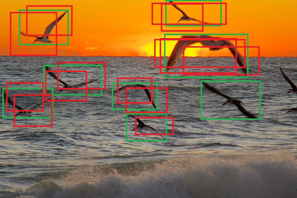
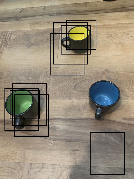
But, before non-maximum suppression, the predictions typically look something like the below.
Feb 19, 2015 - morning sunrise, 02 by Ed Yourdon is licensed under CC BY-NC-SA 2.0
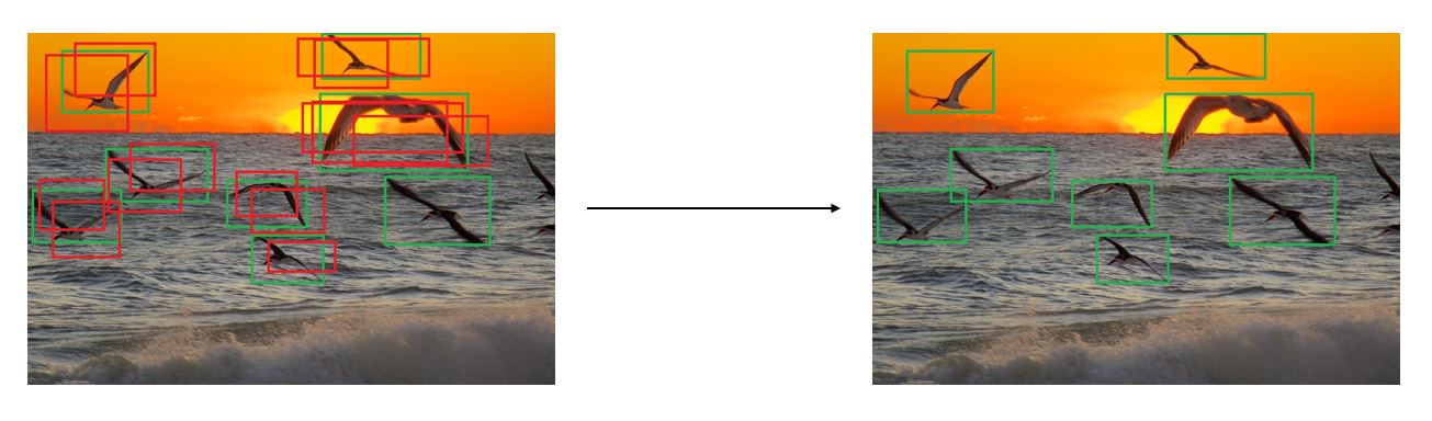
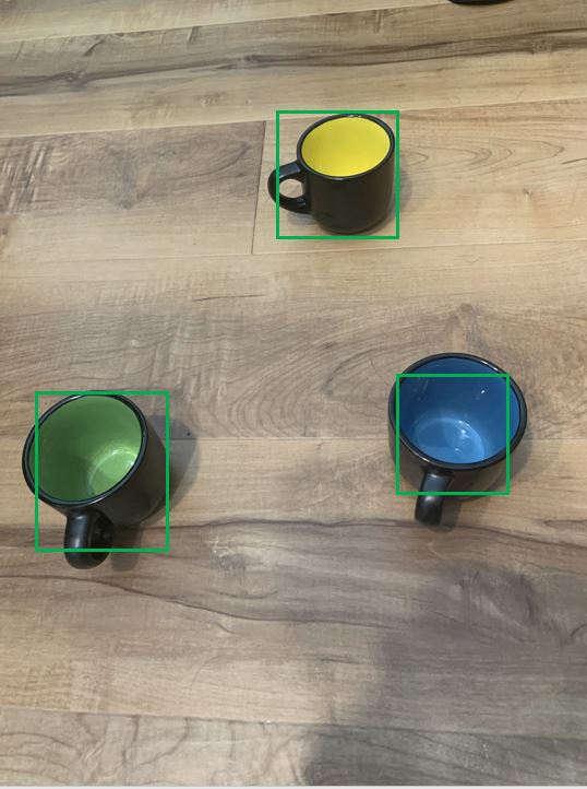
What non-maximum suppression does is take us from a raw model output that has false positives to a refined model output
with only one bounding box per object.
Feb 19, 2015 - morning sunrise, 02 by Ed Yourdon is licensed under CC BY-NC-SA 2.0
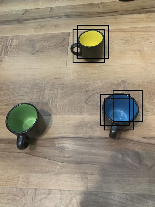
Although non-maximum suppression (NMS) does significantly reduce the number of bounding boxes and typically provides a
satisfactory result, it is an expensive algorithm. Greedy NMS compares each bounding box against
every other bounding box in the image. In our example, we have 22 predictions (8 correct predictions and 14 false positives).
In order to compare each bounding box against every other bounding box, we need to perform (n^2 - n) / 2 comparisons.
In our case, that would be (22 ^ 2 - 22) / 2 operations (where N represents the number of bounding boxes being evaluated),
which comes out to 231 comparisons. As we scale up n, the number of comparisons becomes very large very fast.
Feb 19, 2015 - morning sunrise, 02 by Ed Yourdon is licensed under CC BY-NC-SA 2.0
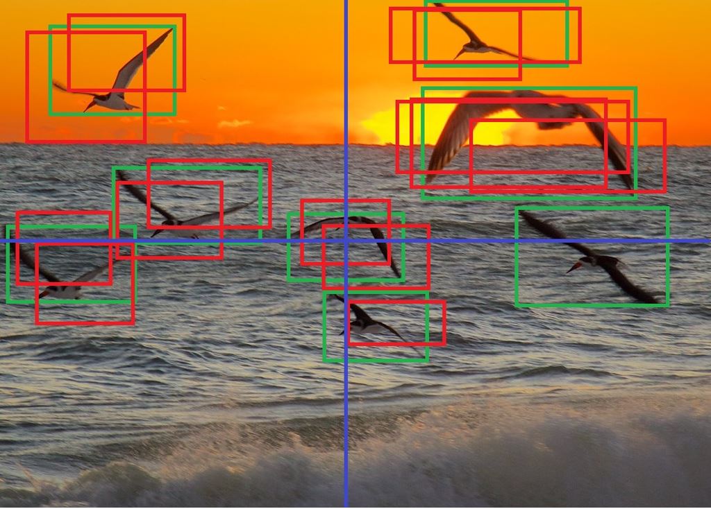
One alternative is to use a "sector-based" approach (SB-NMS). With this approach, instead of comparing each image to every other
image, we divide our image up into "sectors", by recursively splitting it in half. In our example, we have decided to
bisect our image twice into four sectors. This results in M + 2NM + (M + 1) * (N/M) ^ 2 operations (where N represents
the number of bounding boxes being evaluated and M represents the number of sectors that our image has been split
into). This assumes a roughly equal distribution of images over sectors. In reality, the actual efficiency of this
algorithm will be somewhere between slightly slower than Greedy NMS (in worst case scenarios) and up to around 80%
faster than Greedy-NMS in more optimistic scenarios.
Feb 19, 2015 - morning sunrise, 02 by Ed Yourdon is licensed under CC BY-NC-SA 2.0
Note that in our simplified example, with 22 total bounding boxes, Greedy NMS performs fewer operations than SB-NMS and is more efficient. SB-NMS becomes more (theoretically) efficient than Greedy NMS at about 50 total bounding boxes being evaluated (which is far lower than what object detectors typically predict).
In this example, we can see that Greedy NMS makes 231 comparisons. SB-NMS makes 202 comparisons. Although SB-NMS makes fewer comparisons, it does have some up-front costs (e.g. creating sectors, assigning boxes to sectors), which makes it worthwhile only after 50 bounding boxes in its current state.
Theoretical Number of Operations at Different Numbers of Bounding Boxes
| Number of Bounding Boxes | Operations Greedy-NMS | Operations SB-NMS | Approximate Reduction in Operations |
|---|---|---|---|
| 50 | 1,225 | 1,160 | 0% |
| 100 | 4,950 | 3,015 | 40% |
| 500 | 124,750 | 32,618 | 74% |
| 1,000 | 499,500 | 96,259 | 80% |
Actual Performance Comparisons at Different Numbers of Bounding Boxes
To be completed...
We then identify which bounding boxes are overlapping with boundaries.
Feb 19, 2015 - morning sunrise, 02 by Ed Yourdon is licensed under CC BY-NC-SA 2.0
Additionally, we also identify any bounding boxes that overlap with any of our boundary-intersecting bounding boxes. Our first set of selected bounding boxes is picked from these boxes using Greedy NMS. After this round of selecting bounding boxes, the candidate boxes are then removed from consideration from downsteram comparisons. This guarantees that all of the remaining boxes will fall entirely within a single sector.
Note, that the above means SB-NMS prioritizes bounding boxes that fall on boundaries.
Feb 19, 2015 - morning sunrise, 02 by Ed Yourdon is licensed under CC BY-NC-SA 2.0
Next, we iterate over each sector and perform Greedy NMS on the bounding boxes in each sector. We append the results of each iteration of Greedy NMS to our existing set of selected boxes. At the end of the entire process, we end up with a full set of selected bounding boxes.
Typically, Non-Maximum Suppression is run on a single image. When performing object detection on images, many camera factors, like lighting, focus, contrast, play a role in the number of correct detections an object detection model is able to make. Even subtle changes, which can be imperceptible to the human eye, can have an effect on a model's performance, and can lead to decreases in model precision and recall.
Consensus-Based Non-Maximum Suppression Selection (consensus-based-selection) uses a burst of multiple photos of the same subject, from the same angle at approximately the same time (think of taking a burst of 3 images from you phone in 1 second).
Consensus-based selection then performs Non-Maximum Suppression on each photo individually (possibly using Sector-Based Non-Maximum Suppression...), layers the suppressed predictions onto each other (forming a single image of predictions). Then an ensemble of predictions is taken where overlapping bounding boxes boost "confidence", while any singleton predictions (that do not overlap with any other images) are considered random noise and ignored.
Lastly, the remaining predictions are reduced once again. This is done by taking the average (or median, or another measure) of each point of each set of overlapping boxes.
A couple of notes here:
- This methodology works best for real-life scenarios with unreliable lighting. Taking photos outdoors is an excellent example of this. From second-to-second, there can be changes to the lighting that throw off some model predictions, but also make some other model predictions more reliable. Consensus-based selection operates off of the assumption that ensembling these unreliable predictions can yield a much more powerful prediction.
- The obvious first choice to boost model performance is to create a better object detection model (possibly with image augmentation for the abnormal lighting/camera scenarios). In many cases it's either not doable (possibly due to not being in control of the model), prohibitively expensive (either in terms of money or training time), or the model has just plateaued in terms of performance (i.e. it does not respond augmentation or other changes). In these scenarios, consensus-based selection makes sense.
- There is a tradeoff here. As we add more images (which adds more predictions to our ensemble), we add more compute onto our system. If speed of prediction is not paramount, then this is not a problem. If speed of prediction is important, then using a smarter Non-Maximum Suppression algorithm (like Sector-Based Non-Maximum Suppression) is very useful.
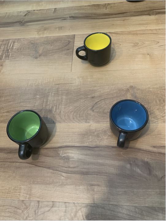
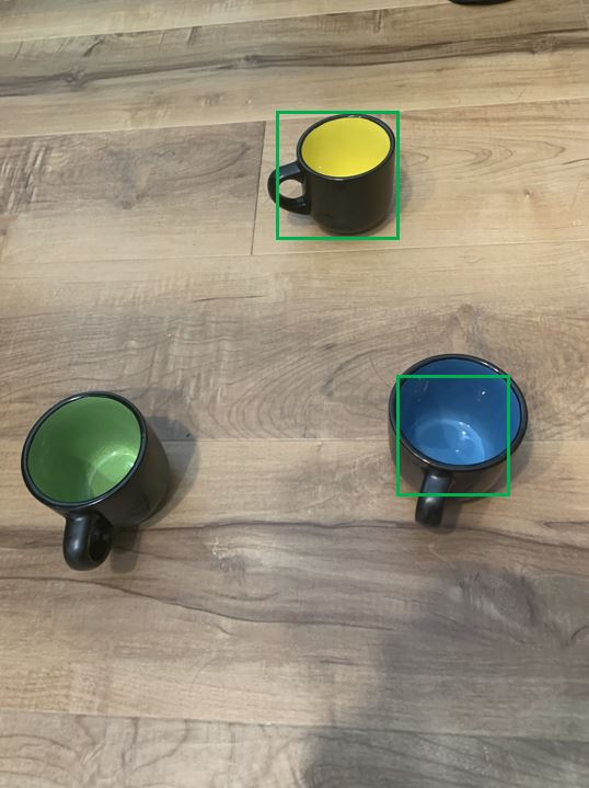
We are going to take a photo of the following subject to pass through our object detection model:
Copyright 2020 - Michael Hernandez
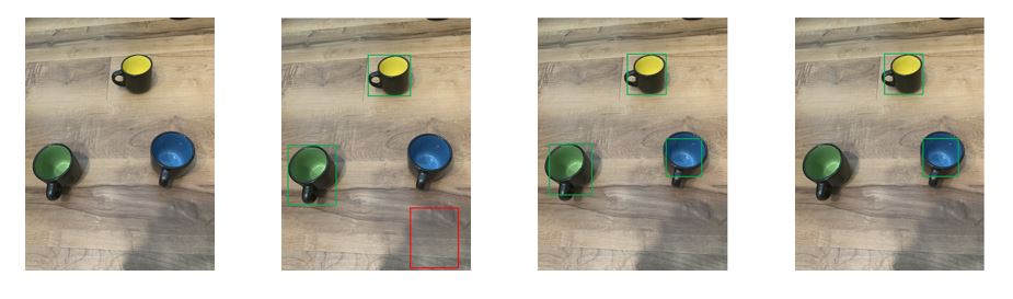
Instead of taking a single picture, we take a burst of 3 (this number can be scaled to fit the user's needs) images in a row:
Copyright 2020 - Michael Hernandez
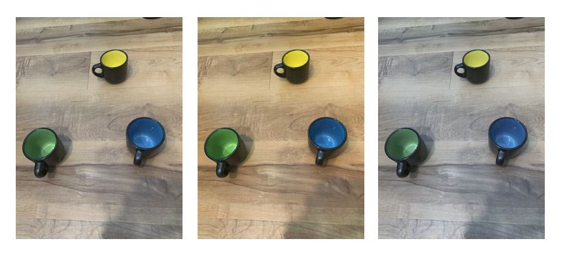
As we can see above, due to different lighting (exaggerated in this case), we get three photos of the same subject from the same angle, but with slight differences. In real life scenarios with unreliable lighting (e.g. outdoors, indoor flickering lighting) or an unreliable camera (e.g. some phone cameras, unsteady holding of camera) images will have minor imperfections which can change moment-to-moment.
Note: For the rest of this example, we'll be showing un-distorted images for simplicity
Our first step in Consensus-Based Non-Maximum Suppression Selection is to perform Non-Maximum Suppression on our images in isolation.
Raw predictions for first image:
Copyright 2020 - Michael Hernandez
Suppressed predictions for first image:
Copyright 2020 - Michael Hernandez

Raw predictions for second image:
Copyright 2020 - Michael Hernandez
Suppressed predictions for second image:
Copyright 2020 - Michael Hernandez
Raw predictions for third image:
Copyright 2020 - Michael Hernandez
Suppressed predictions for third image:
Copyright 2020 - Michael Hernandez
As a result, we now have the following filtered predictions after performing non-maximum suppression:
Copyright 2020 - Michael Hernandez
Since our predictions are of the same subject from the same angle (at approximately the same time), we can layer the
predictions on top of each other:
Copyright 2020 - Michael Hernandez
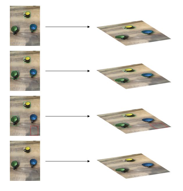
After layering, we can flatten all of the predictions down to a single layer (the bottom layer in the image is simply the original with no predictions):
Copyright 2020 - Michael Hernandez
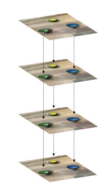
After flattening, we get the resulting image with the following predictions upon which we calculate the intersection
over the union (IOU) for each pair of boxes (only non-zero IOU values are shown):
Copyright 2020 - Michael Hernandez
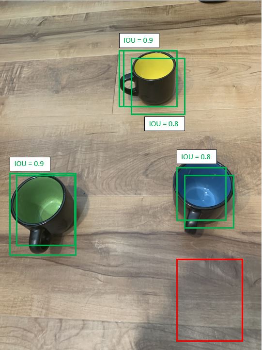
We then select a threshold value that each IOU must exceed in order for two boxes to be grouped together (i.e. boxes
that are of the same subject):
Copyright 2020 - Michael Hernandez
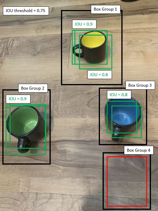
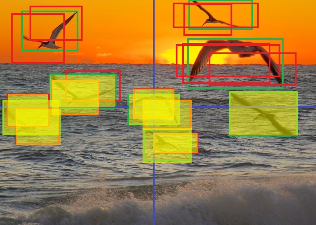
Next, we ensemble these predictions together. Since we have 3 images worth of predictions, any box group that contains
a majority (i.e. 2) boxes will retain its predictions. All other box groups will be removed:
Copyright 2020 - Michael Hernandez
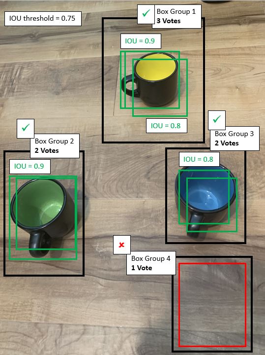
Now that ensembling has taken place, we are only left with three box groups' worth of predictions:
Copyright 2020 - Michael Hernandez

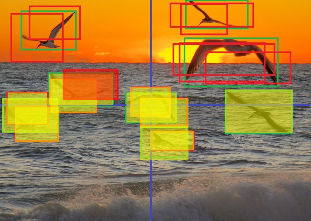
The final step is to remove any excess boxes. This can be done in a variety of ways. For this example, since we already
know which boxes overlap, we can actually take the average (or median) point of each corner and use that as the corners
of our resulting bounding boxes. That results in the following yellow bounding boxes:
Copyright 2020 - Michael Hernandez
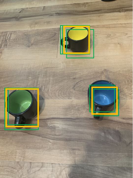
And after removing the old bounding boxes we are left with only the correct ones:
Copyright 2020 - Michael Hernandez
Installation:
python setup.py installQuick Start:
The first step is to get some bounding box predictions to process. All bounding boxes must be measured in relative coordinates (i.e. scaled from 0 to 1). In this example, we will be creating four bounding boxes. Note that all labels have already been encoded.
import numpy as np
boxes = np.array((
    ((0.190146, 0.241815), (0.405093, 0.409226)),
    ((0.595238, 0.074405), (0.892857, 0.262897)),
    ((0.644841, 0.520833), (0.975529, 0.725446)),
    ((0.941701, 0.991324), (0.110437, 0.241192))
))

confidences = np.array((0.65, 0.89, 0.70, 0.14))

labels = np.array((0, 1, 1, 1))
In this example, we'll be simulating having multiple ("n_boxes") overlapping bounding boxes by jittering the coordinates of our three ground truth boxes.
n_boxes = 5  # The number of boxes to simulate per original box.
std = 0.005  # The standard deviation for normal random sampling.
new_boxes = []
new_confidences = []
new_labels = []
for i in range(n_boxes):
    for j in range(boxes.shape[0]):
        print(f"Adding new box {i} around existing box {j}")
        new_box_pt1_x = boxes[j, 0, 0] + np.random.normal(loc=0, scale=std)
        new_box_pt1_y = boxes[j, 0, 1] + np.random.normal(loc=0, scale=std)
        new_box_pt2_x = boxes[j, 1, 0] + np.random.normal(loc=0, scale=std)
        new_box_pt2_y = boxes[j, 1, 1] + np.random.normal(loc=0, scale=std)
        new_box = np.array(((new_box_pt1_x, new_box_pt1_y), (new_box_pt2_x, new_box_pt2_y)), dtype=np.float64)
        new_boxes.append(new_box)
        new_confidence = confidences[j] + np.random.uniform(-0.1, 0.1)
        new_confidences.append(new_confidence)
        new_labels.append(labels[j])

new_boxes.append(boxes)
boxes = np.concatenate(new_boxes, axis = 0)
In most cases, we will want to filter out bounding boxes below our confidence threshold before applying our non-maximum suppression algorithm. Here, we are filtering out the bounding boxes below 50% confidence.
confidence_threshold = 0.5
confidences = confidences[confidences > confidence_threshold]
labels = labels[confidences > confidence_threshold]
boxes = boxes[confidences > confidence_threshold]
Now that we have a set of boxes to run out non-maximum suppression algorithm on, we can create instances of our metric and selector. We can then pass those onto our suppression algorithm, along with our iou_threshold value. Once we have an instance of our suppression algorithm, we run the transform() method to apply non-maximum suppression.
import od_toolbelt as od

# All pairs of bounding boxes with intersection over the union of 0.25 or less will be considered separate boxes.
METRIC_THRESHOLD = 0.25

metric = od.nms.metrics.DefaultIntersectionOverTheUnion(threshold=METRIC_THRESHOLD, direction="lte")
selector = od.nms.selection.RandomSelector()

nms = od.nms.suppression.CartesianProductSuppression(
    metric=metric, selector=selector
)

data_payload = od.BoundingBoxArray(
    bounding_boxes=boxes,
    confidences=confidences,
    labels=labels,
)

resulting_payload = nms.transform(data_payload)
Alternatively, we can use other non-maximum suppression algorithms, such as the SectorSuppression algorithm. We can runt he same transform() method.
sector_divisions = 1
nms = od.nms.suppression.SectorSuppression(
    metric=metric, selector=selector, sector_divisions=sector_divisions
)

resulting_payload = nms.transform(data_payload)
Also, note that the metric and selector can be changed out for others (or use-defined metrics and selectors).
Suppressors are our non-maximum suppression algorithms. They are what developer creates and runs in order to apply non-maximum suppression.
They are inherited off of a base class. To use them, the developer should create an instance of a suppressor class.
Metrics are how we measure the degree to which two bounding boxes overlap. Intersection over the union is one such metric, but other metrics can be used as well. To use them, the developer should create an instance of a metric class.
After creating an instance of a metric class, the developer simply needs to pass two bounding boxes to the compute() method. A float metric value is returned.
Selectors are how non-maximum suppression algorithms select a single bounding box from many. Random selection is one such selector, but other selectors can be used as well. To use them, the developer should create an instance of a selector class.
After creating an instance of a selector class, the developer simply needs to pass a list of bounding box identifiers to the select() method. A single identifier is returned.
Aggregators are how multiple images' worth of suppressed bounding boxes are aggregated down to a single set of bounding boxes. To use them, the developer should first run non-maximum suppression on a burst of images.
- Python code optimizations.
- Add consensus-based aggregator.
- Add additional selectors (e.g. first selector, average selector, median selector, etc.).
- Add additional metrics (e.g. IOU^2, etc.).
- Complete refactorization.
- Create PyPi package.
- Convert codebase to optimized Cython.
- Add soft-NMS as an option.
- Integration with object detection frameworks (e.g. Tensorflow, etc.).
- Integration with object detection services (e.g. AWS SageMaker, Azure Custom Vision, etc.).