This was the template for one of my theses at the TU Darmstadt.
- How to use
- Features
- To-do notes
- Colors for corporate design
- Tables
- Equations
- List of Acronyms
- List of Symbols
- Beautiful graphs
- Text replacement
- Electronic circuits
- Custom styled bibliography
- Acknowledgements
-
Download tud-design packages from the physics department
-
Download the fonts for corporate design. You need a student account for the university in order to download the fonts. This step is optional. Template will also work without the fonts
-
Install the packages as described in the manual
-
Edit the template from this repo according to your needs
-
Run
latex -
Run
makeglossaries thesisfrom the command line to sort and typeset glossaries and list of acronyms/symbols -
Run
biblatex -
Run
latexfor the last time and enjoy the output
All features can be used in any LaTeX document and don't depend on the tud classes.
Very useful while writing the thesis. Don't forget to delete them before printing the final copy. Enable to-do notes with the todonotes package. I usually use the inline style.
\usepackage[ngerman]{todonotes}
\todo[inline]{This is a sample to-do note}
Print a list with your open to-do notes using the following command.
\listoftodos
Define your own colors for later use in graphs or text.
\definecolor{blue_1a}{RGB}{93,133,195}
\definecolor{green_3a}{RGB}{80,182,149}
\definecolor{red_8a}{RGB}{238,122,52}
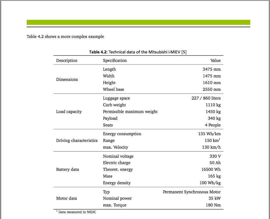
For tables I used the ctable package. It allows to specify a seperate caption for the toc and therefore enables citations inside the table's caption. It also allows us to write footnotes directly below the table to further explain certain facts.
\ctable[
	caption = Technical data of the Mitsubishi i-MiEV \cite{imiev_daten},
	cap = Technical Data of the Mitsubishi i-MiEV,
	label	= tab:data_imiev,
	pos = htb
	]{llr}
	{\tnote[1]{Data measured in NEDC}}
	{\FL Description & Specification & Value
		\ML \multirow{4}*{Dimensions} & Length & 3475 mm
		\NN & Width & 1475 mm
		\NN & Height & 1610 mm
		\NN & Wheel base & 2550 mm
		\ML \multirow{5}*{Load capacity} & Luggage space & 227 / 860 liters
		\NN & Curb weight & 1110 kg
		\NN & Permissible maximum weight & 1450 kg
		\NN & Payload & 340 kg
		\NN & Seats & 4 People
		\ML \multirow{3}*{Driving characteristics} & Energy consumption & 135 Wh/km
		\NN & Range & 150 km\tmark[1]
		\NN & max. Velocity & 130 km/h
		\ML \multirow{5}*{Battery data} & Nominal voltage & 330 V
		\NN & Electric charge & 50 Ah
		\NN & Theoret. energy & 16500 Wh
		\NN & Mass & 165 kg
		\NN & Energy density & 100 Wh/kg
		\ML \multirow{3}*{Motor data} & Typ & Permanent Synchronous Motor
		\NN & Nominal power & 35 kW
		\NN & max. Torque & 180 Nm
		\LL}
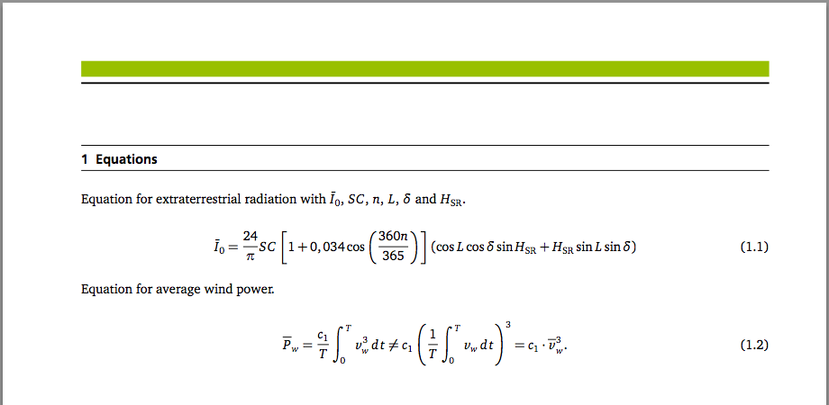
The big advantage of LaTex is how nicely complex equations are handled.
Equation for extraterrestrial radiation. Taken from Renewable and Efficient Electric Power Systems by Gilbert M. Masters on page 432, 7.43.
\begin{equation}
  \glsentrytext{I0} = \frac{24}{\pi} \glsentrytext{SC} \left[1+0,034\cos\left(\frac{360\glsentrytext{n}}{365}\right)\right](\cos \glsentrytext{L} \cos \glsentrytext{delta} \sin \glsentrytext{HSR} + \glsentrytext{HSR} \sin \glsentrytext{L} \sin \glsentrytext{delta})
\end{equation}
Equation for average wind power. Taken from Betrieb von Kleinwindkraftanlagen - ein Überblick über Markt, Technik und Wirtschaftlichkeit by W. Halbhuber on page 95.
\begin{equation}
	\overline P_w = \frac{c_1}{T} \int_0^T v_w^3\,dt \ne c_1 \left(\frac{1}{T}\int_0^T v_w\,dt\right)^3 = c_1 \cdot \overline{v}_w^3.
\end{equation}
Define your acronyms.
\newacronym{CO2}{CO\ensuremath{_\textnormal{2}}}{Carbon dioxide}
\newacronym{NEDC}{NEDC}{New European Driving Cycle}

% Print acronyms
\printglossary[type=acronym, title=Acronyms, toctitle=Acronyms, style=mystyle]
Add an optional custom style
% Define custom style for glossaries
\newglossarystyle{mystyle}{%
  % full stop after every description
	\renewcommand*{\glspostdescription}{}%
	% put the glossary in a longtable environment:
  % left alignment, no white in front und three columns
	\renewenvironment{theglossary}{\begin{longtable}[l]{@{}lcl}}{\end{longtable}}
	% have nothing after \begin{theglossary}:
	\renewcommand*{\glossaryheader}{}%
  % uncomment following line if you want headings
	% \renewcommand*{\glossaryheader}{\bfseries Symbol & \bfseries Unit & \bfseries Description \endhead}%
	% have nothing between glossary groups (next two commands):
	\renewcommand*{\glsgroupheading}[1]{}%
	% Suppress the vertical gap at the start of each group
	\renewcommand*{\glsgroupskip}{}%
	% set how each entry should appear:
	\renewcommand*{\glossaryentryfield}[5]{%
		\glstarget{##1}{##2}	% Name
		& ##4					        % Symbol
		& ##3					        % Description
		% & ##5					      % Page list
		\\% end of row
	}%
	% Sub entries treated the same as level 0 entries:
	\renewcommand*{\glossarysubentryfield}[6]{%
		\glossaryentryfield{##2}{##4}{##3}
	}%
}
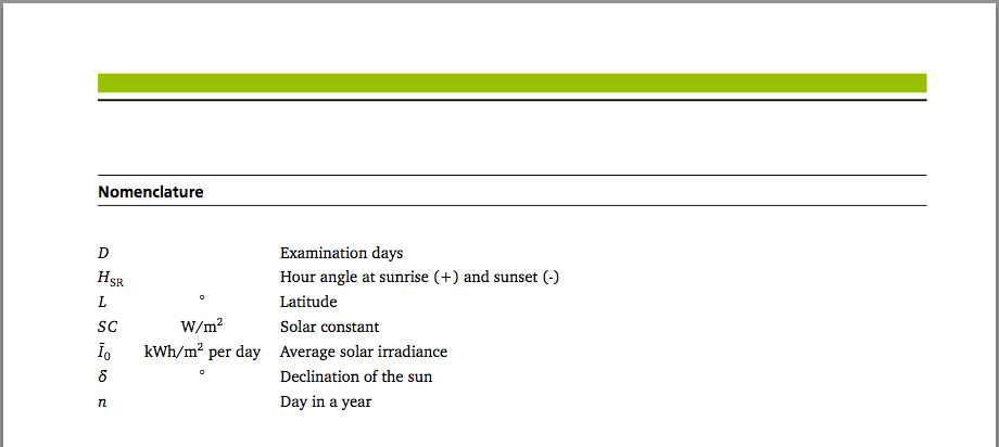
\newglossaryentry{D}{name=\ensuremath{D}, symbol={}, description={Examination days}, type=symbolslist}
\newglossaryentry{I0}{name=\ensuremath{\bar I_{\textnormal{0}}}, symbol={kWh/m\ensuremath{^2} per day}, description={Average solar irradiance}, type=symbolslist}
\newglossaryentry{SC}{name=\ensuremath{SC}, symbol={W/m\ensuremath{^2}}, description={Solar constant}, type=symbolslist}
\newglossaryentry{n}{name=\ensuremath{n}, symbol={}, description={Day in a year}, type=symbolslist}
\newglossaryentry{L}{name=\ensuremath{L}, symbol={\ensuremath{^\circ}}, description={Latitude}, type=symbolslist}
\newglossaryentry{delta}{name=\ensuremath{\delta}, symbol={\ensuremath{^\circ}}, description={Declination of the sun}, type=symbolslist}
\newglossaryentry{HSR}{name=\ensuremath{H_{\textnormal{SR}}}, symbol={}, description={Hour angle at sunrise (+) and sunset (-)}, type=symbolslist}

% Print list of symbols
\printglossary[type=symbolslist, style=mystyle]
\begin{figure}[htb]
\centering
\begin{tikzpicture}
\begin{axis}[
xlabel= Wind speed in m/s,
ylabel= Relative frequency in \%,
xmin = 0,
xmax = 25,
ymin = 0,
ymax = 30,
width= 120mm,
height = 80mm,
%legend columns=-1,
axis x line = bottom,
axis y line = left,
legend style = {draw = none, cells={anchor=west}}
]
\addplot+[mark=none, blau_2b, very thick] file {data/weibull_k1.dat};
\addplot+[mark=none, gruen_4b, very thick] file {data/weibull_k1_5.dat};
\addplot+[mark=none, orange_6b, very thick] file {data/weibull_k2.dat};
\addplot+[mark=none, rot_8b, very thick] file {data/weibull_k3.dat};
\legend{k=1, {k=1,5}, k=2, k=3}
\end{axis}
\end{tikzpicture}
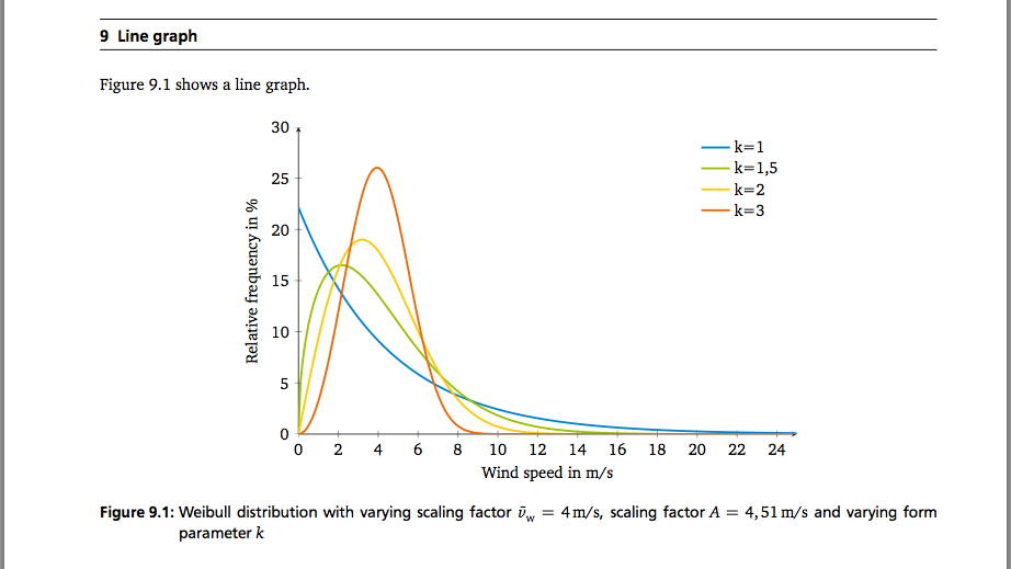
\caption[Weibull distribution with varying scaling factor]{Weibull distribution with varying scaling factor $\bar v_\textnormal{w} = 4\,\textnormal{m/s}$, scaling factor $A = 4,51\,\textnormal{m/s}$ and varying form parameter $k$}
\label{fig:weibull_distribution}
\end{figure}
\begin{figure}[htb]
\centering
\begin{tikzpicture}
\begin{axis}[
ybar,
xlabel = Month,
xmin = 0.5,
xmax = 13.5,
ymin = 0,
ymax = 35,
axis x line* = bottom,
axis y line* = left,
ylabel= New electric vehicles,
width= 0.9\textwidth,
height = 0.6\textwidth,
ymajorgrids = true,
bar width = 5mm,
xticklabels = \empty,
extra x ticks = {1,2,3,4,5,6,7,8,9,10,11,12,13},
extra x tick labels = {Jan '09, Feb, Mar, Apr, May, Jun, Jul, Aug, Sep, Oct, Nov, Dec, Jan '10},
]
\addplot+[mark=none, blau_2b, very thick] coordinates {
(1,3)
(2,3)
(3,7)
(4,1)
(5,28)
(6,13)
(7,4)
(8,7)
(9,4)
(10,14)
(11,10)
(12,18)
(13,35)
};
\end{axis}
\end{tikzpicture}
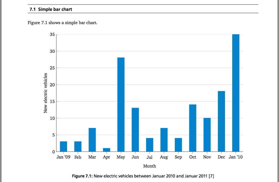
\caption[New electric vehicles between Januar 2010 and Januar 2011]{New electric vehicles between Januar 2010 and Januar 2011 \cite{sa-neuzulassungen}}
\label{fig:new_ev}
\end{figure}
\begin{figure}[htb]
\centering
\begin{tikzpicture}
\begin{axis}[
ybar stacked,
xlabel= Year,
ylabel = Energy in GWh,
ymajorgrids = true,
width = 0.9\textwidth,
height = 0.5\textwidth,
xmin = 1999.5,
xmax = 2009.5,
ymin = 0,
ymax = 70000,
axis x line* = bottom,
axis y line* = left,
xticklabels = none,
extra x ticks = {2000, 2001, 2002, 2003, 2004, 2005, 2006, 2007, 2008, 2009},
extra x tick labels = {2000, 2001, 2002, 2003, 2004, 2005, 2006, 2007, 2008, 2009},
legend style = {at={(0.5, 1.025)}, anchor = south, legend columns = -1, draw=none, area legend},
area legend,
scaled ticks = false,
y tick label style = {/pgf/number format/use comma}
]
\addplot+[mark=none, fill=blau_2b, draw = blau_2b, bar width = 8mm] table[x=year, y=ror] {data/stacked-bar-chart.dat};
\addplot+[mark=none, fill=lila_10b, draw = lila_10b, bar width = 8mm] table[x=year, y=storage] {data/stacked-bar-chart.dat};
\addplot+[mark=none, fill=orange_6b, draw = orange_6b, bar width = 8mm] table[x=year, y=thermal] {data/stacked-bar-chart.dat};
\addplot+[mark=none, fill=gruen_4b, draw = gruen_4b, bar width = 8mm] table[x=year, y=renewable] {data/stacked-bar-chart.dat};
\legend{\gls{ROR}, Storage power plant, Thermal power station, Renewable energy}
\end{axis}
\end{tikzpicture}
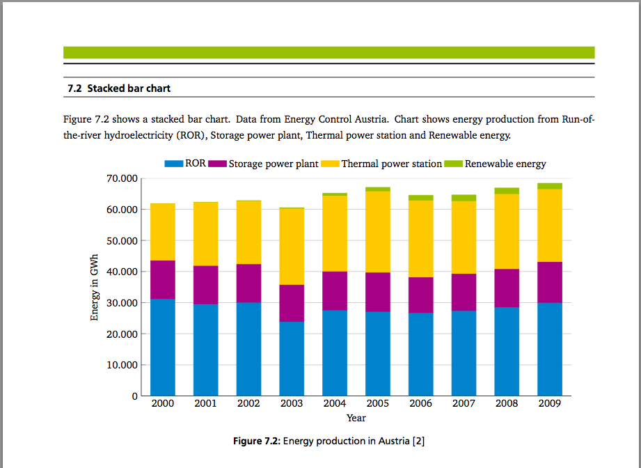
\caption[Energy production in Austria]{Energy production in Austria \cite{econtrol2011}}
\label{fig:energy_austria}
\end{figure}
\newcommand{\slice}[4]{
\pgfmathparse{0.5*#1+0.5*#2}
\let\midangle\pgfmathresult
% slice
\draw[thick] (0,0) -- (#1:1) arc (#1:#2:1) -- cycle;
% outer label
\node[label=\midangle:#4] at (\midangle:1) {};
% inner label
\pgfmathparse{min((#2-#1-10)/110*(-0.3),0)}
\let\temp\pgfmathresult
\pgfmathparse{max(\temp,-0.5) + 0.8}
\let\innerpos\pgfmathresult
\node at (\midangle:\innerpos) {#3};
}
\begin{figure}[htb]
\centering
\begin{tikzpicture}[scale=3]
\newcounter{a}
\newcounter{b}
\foreach \p/\t in {5/Shot break, 19/Rotor, 7/Gear + Generator, 18/remaining Housing, 20/Tower, 6/Power connection, 8/Basement, 3/Misc, 14/Operation}
{
\setcounter{a}{\value{b}}
\addtocounter{b}{\p}
\slice{\thea/100*360}
{\theb/100*360}
{\p\%}{\t}
}
\end{tikzpicture}
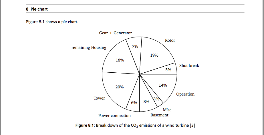
\caption[Break down of the CO$_2$ emissions of a wind turbine]{Break down of the CO$_2$ emissions of a wind turbine \cite{kaltschmitt2006}}
\label{fig:co2_wind}
\end{figure}
\begin{figure}[htb]
\centering
\begin{tikzpicture}
\begin{axis}[
ybar,
scale only axis,
xlabel= Trips in 2010,
width = 0.8\textwidth,
height = 0.5\textwidth,
ylabel= Covered distance in km,
% height = 80mm,
ymin = 0,
ymax = 800,
xmin = 0,
xmax = 111,
bar width = 0.5mm,
axis x line* = bottom,
axis y line* = left,
bar shift = -0.25mm,
y tick label style = {/pgf/number format/use comma},
legend style = {at={(0.5, 1.025)}, anchor = south east, legend columns = -1, draw=none, area legend},
area legend
]
\addplot+[mark=none, blau_2b] table[x=number, y=km] {data/ev.dat};
\addplot+[line legend, sharp plot, dashed, line width = 2pt, mark=none, draw = blau_2b] coordinates{(0,150) (111,150)};
\legend{Kilometers, max. range (150 km)}
\end{axis}
\begin{axis}[
ybar,
scale only axis,
width = 0.8\textwidth,
height = 0.5\textwidth,
axis y line* = right,
axis x line = none,
ylabel = Immobilization time between two trips in hours,
% height = 80mm,
xmin = 0,
xmax = 111,
ymin = 0,
ymax = 410,
bar width = 0.5mm,
bar shift = 0.25mm,
legend style = {at={(0.5, 1.025)}, anchor = south west, legend columns = -1, draw=none, area legend},
area legend
]
\addplot+[mark=none, gruen_4b] table[x=number, y=time] {data/ev.dat};
\addplot+[line legend, sharp plot, dashed, line width = 2pt, mark=none, draw = gruen_4b] coordinates{(0,8) (111,8)};
\legend{Immobilization time, Charging time (8h)}
\end{axis}
\end{tikzpicture}
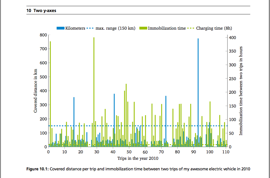
\caption[Covered distance and immobilization time between trips of my awesome electric vehicle]{Covered distance per trip and immobilization time between two trips of my awesome electric vehicle in 2010}
\label{fig:trips_ev}
\end{figure}
Before
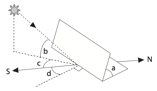
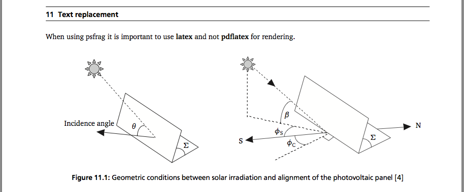
\begin{figure}[htb]
	\centering
	\subfloat{
		\psfrag{a}[c][c]{$\theta$}
		\psfrag{b}[c][c]{$\Sigma$}
		\psfrag{c}[c][c]{Incidence angle}
		\centering
			\includegraphics[width=70mm]{images/collector_theta-01.eps}
	}\hspace{1cm}
	\subfloat{
		\psfrag{S}[c][c]{S}
		\psfrag{N}[c][c]{N}
		\psfrag{a}[c][c]{$\Sigma$}
		\psfrag{b}[c][c]{$\beta$}
		\psfrag{c}[c][c]{$\phi_\textnormal{S}$}
		\psfrag{d}[c][c]{$\phi_\textnormal{C}$}
		\centering
			\includegraphics[width=90mm]{images/collector_geometry-01.eps}
	}
	\caption[Geometric conditions between solar irradiation and alignment of the photovoltaic panel]{Geometric conditions between solar irradiation and alignment of the photovoltaic panel \cite{masters04}}
	\label{fig:collector}
\end{figure}
After
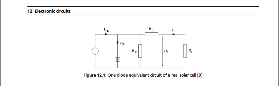
\begin{tikzpicture}[
	circuit ee IEC,
	set inductor graphic=var inductor IEC graphic,
	scale = 0.85,
	]
	\draw (0,0) to [current source] (0,3);
	\draw (0,3) to [current direction={info=$I_\textnormal{Ph}$}] (2,3);
	\draw (2,3) -- (4,3);
	\draw (2,3) to [current direction={info={$I_\textnormal{D}$}}] (2,1.5) to [diode] (2,0);
	\draw (0,0) to (8,0);
	\draw (4,0) to [resistor={info={$R_\textnormal{P}$}}] (4,3);
	\draw (4,3) to [resistor={info={$R_\textnormal{S}$}}] (6,3);
	\draw (6,3) to [current direction={info={$I_\textnormal{L}$}}] (8,3);
	\draw (8,3) to [resistor={info={$R_\textnormal{L}$}}](8,0);
	\draw [->] (6,2.8) -- (6,0.2);
	\draw (6,1.5) node[anchor=west]{$U_\textnormal{L}$};
\end{tikzpicture}
Before
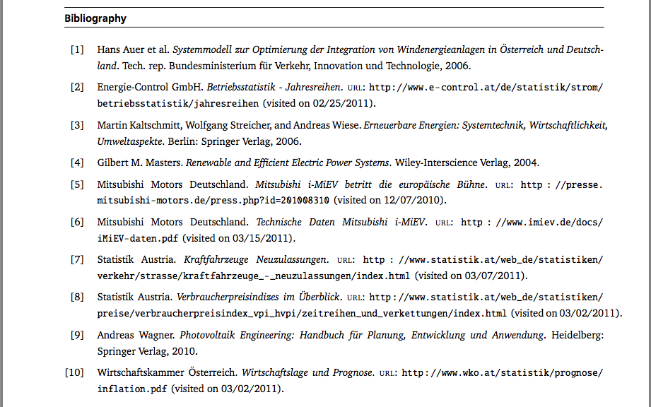
\usepackage[style=numeric, firstinits=true, backend=bibtex]{biblatex}
\urlstyle{same}
\DeclareFieldFormat{title}{#1\isdot}
\renewcommand{\labelnamepunct}{\addcolon\space}
\renewcommand{\multinamedelim}{\addsemicolon\space}
\renewcommand{\finalnamedelim}{\addsemicolon\space}
\DeclareNameFormat{default}{\usebibmacro{name:last-first}{#1}{#4}{#5}{#7}\usebibmacro{name:andothers}}
\DefineBibliographyStrings{ngerman}{urlseen={abgerufen am}}

\bibliography{bibliography/bibliography}
After

Clemens v. Loewenich and Johannes Werner for creating the tud classes.