##Writeup Template ###You can use this file as a template for your writeup if you want to submit it as a markdown file, but feel free to use some other method and submit a pdf if you prefer.
Advanced Lane Finding Project
The goals / steps of this project are the following:
- Compute the camera calibration matrix and distortion coefficients given a set of chessboard images.
- Apply a distortion correction to raw images.
- Use color transforms, gradients, etc., to create a thresholded binary image.
- Apply a perspective transform to rectify binary image ("birds-eye view").
- Detect lane pixels and fit to find the lane boundary.
- Determine the curvature of the lane and vehicle position with respect to center.
- Warp the detected lane boundaries back onto the original image.
- Output visual display of the lane boundaries and numerical estimation of lane curvature and vehicle position.
Rubric Points
###Here I will consider the rubric points individually and describe how I addressed each point in my implementation.
###Writeup / README
###Camera Calibration
####1. Briefly state how you computed the camera matrix and distortion coefficients. Provide an example of a distortion corrected calibration image.
I created a class called Camera which has the main task of calibrating the camera and offers an undistort function to remove radial and tangential radiation from images.
I start by preparing "object points", which will be the (x, y, z) coordinates of the chessboard corners in the world.
Here I am assuming the chessboard is fixed on the (x, y) plane at z=0, such that the object points are the same for each
calibration image. Thus, objp is just a replicated array of coordinates, and objpoints will be appended with a copy
of it every time I successfully detect all chessboard corners in a test image.
imgpoints will be appended with the (x, y) pixel position of each of the corners
in the image plane with each successful chessboard detection.
I then used the output objpoints and imgpoints to compute the camera calibration and distortion coefficients using
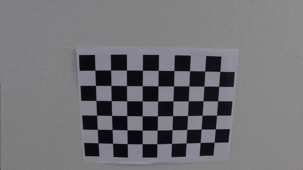
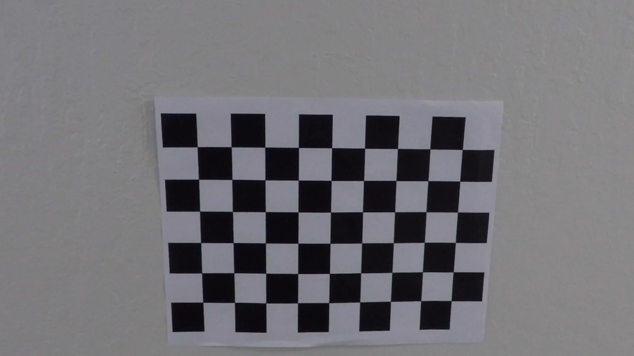
the cv2.calibrateCamera() function. I applied this distortion correction to the test
image using the cv2.undistort() function and obtained this result:
Original Pattern
Undistorted Pattern
###Pipeline (single images)
####1. Provide an example of a distortion-corrected image.
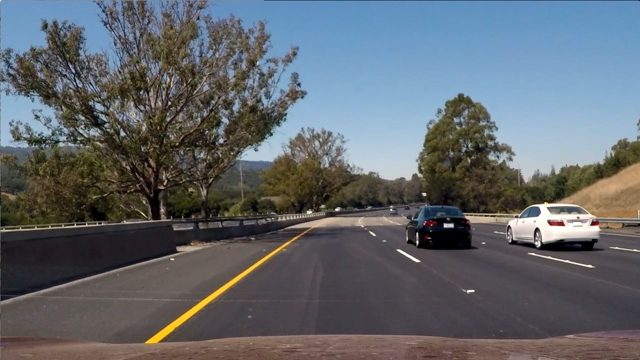
To demonstrate this step, I will describe how I apply the distortion correction to one of the test images like this one:
 ####2. Describe how (and identify where in your code) you used color transforms, gradients or other methods to create a thresholded binary image. Provide an example of a binary image result.
All filtering functions were implemented int he class FilterTools.
A combination of those functions was then used in order to generate an optimal filtered image resulting from the combination of filtered image using different methods, in my case intensity based.
I used:
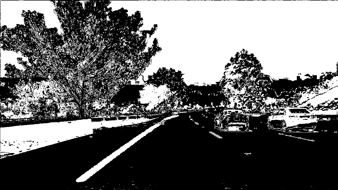
Sobel filter in x and y directions on the S component of the HLS color space Sobel filter in x and y directions on the Gray Image Thresholding the intensity on the S component of the HLS color space Thresholding the intensity on the Gray Image
Then those binary images where combined. This was implemented int he function 'filter'
Here's an example of my output for this step.
This filtering is done on the original image, before the undistorting.
####3. Describe how (and identify where in your code) you performed a perspective transform and provide an example of a transformed image.
The code for my perspective transform includes a function called warp(),
The warp() function takes as inputs a binary filtered image (filtered_img),
as well as color image (original_image).
In my code the perspective warp matrix is defined globally as well as the destination shape
that I chose to be 800x800.
I chose the hardcode the source and destination points in the following manner:
roi = np.float32([[100, 666], [490, 500], [840, 500], [1230, 666]])
# Target bird eye view image shape
warped_shape = np.array([800, 800])
target_roi = np.float32([[0, warped_shape[0]], [0, 0], [warped_shape[0], 0], warped_shape])
This resulted in the following source and destination points:
| Source | Destination |
|---|---|
| 100, 666 | 0, 800 |
| 490, 500 | 0, 0 |
| 840, 500 | 800, 0 |
| 1230, 666 | 800, 800 |
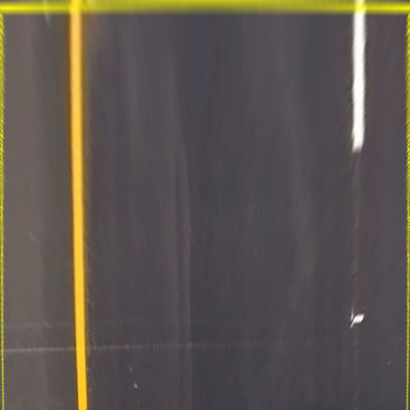
I verified that my perspective transform was working as expected by drawing the region of interest in the original image, then warping that image
Here is the image with its respective region of interest (source points)
When warped one can see that the yellow ROI edges appear indeed parallel so the perspective transform is valid.
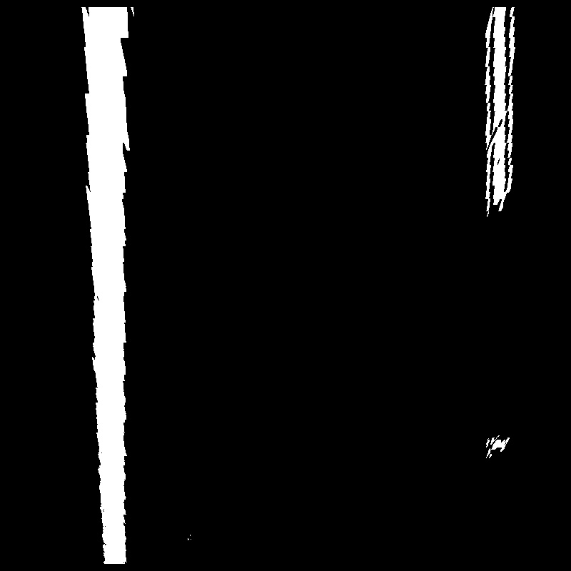
And the result when applying the same warping to the binary image shown above:
####4. Describe how (and identify where in your code) you identified lane-line pixels and fit their positions with a polynomial?
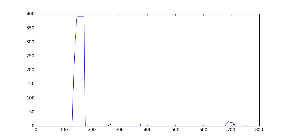
Once the warped binary image is available, I compute a histogram of intensities by summing up all the rows. Expecting lane lines to appear vertical in the warped image, the histogram is expected to have to clearly identifiable maximas. One towards the left of the image and one towards the right of the image.
Here Is an example histogram corresponding to the image above:
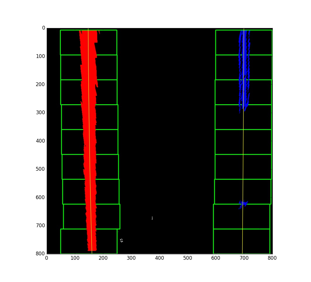
Running the function 'search_for_lines' on this patch returns 2 degrees polynomial fitting to the vertical white blobs found around the histogram maximas. It first starts at the bottom of the image, in a search window around the two peaks of the histogram above then keeps propagating upwards, following the displacement of the white blob.
The following images shows the white blobs detected around histogram maxima (red and blue)
The green rectangles represent the search areas for white pixels. Notices how they are centered around pixels 150 and 700, matching with the peaks of the histogram shown previously. The sliding window method is simple. Start centered and shift left or right depending on the offset between rectangle center and the center of the white blob. If no white pixels are observed, keep the same position and continue with the next rectangle upwards.
The yellow lines are the result of the polynomial fitting. ####5. Describe how (and identify where in your code) you calculated the radius of curvature of the lane and the position of the vehicle with respect to center.
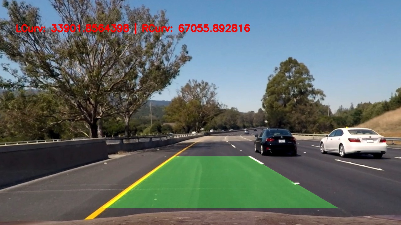
The radius calculation was done as explained in the course, By using the polynomial fit. I kept left and right curve radius separated for debugging reasons. The values I have got made seemed reasonable. The highest radius I have got was in the image with the straight lines. I think here the radius problem is not very well conditioned, and the radius estimation can vary a lot when the lane detection varies a little bit so I assume 100 kilometers here is a good estimation for infinity
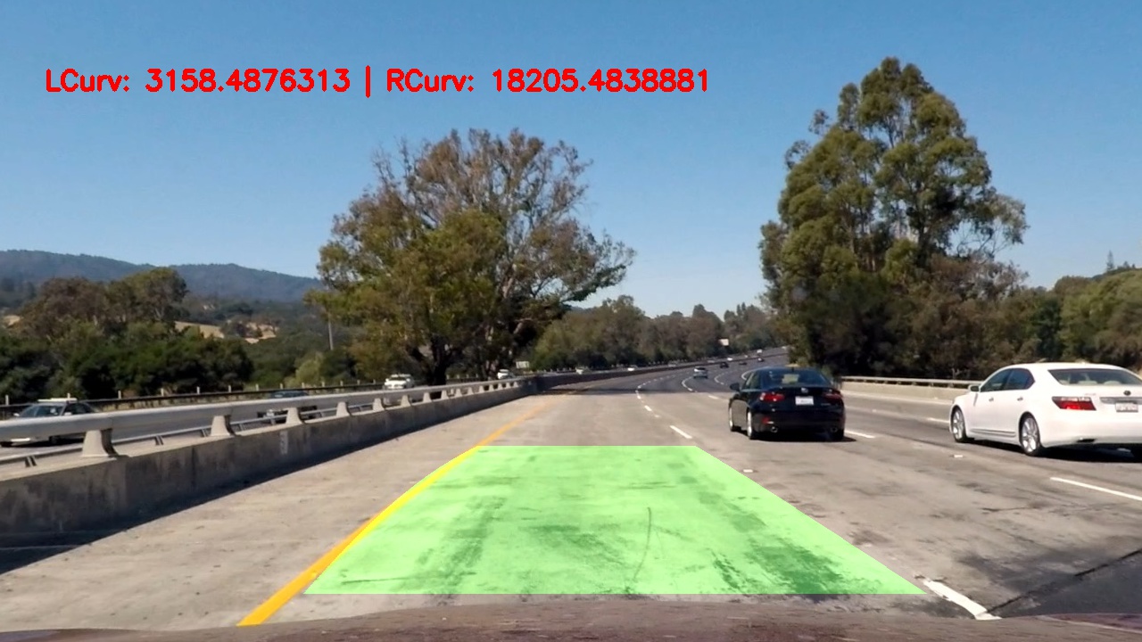
Here is another interesting image where we have curved and non curved lanes
The curved yellow left lane had an estimated curvature radius around 3 kilometers while the nearly straight left lane had a much higher curvature radius (ca. 20 kilometers).
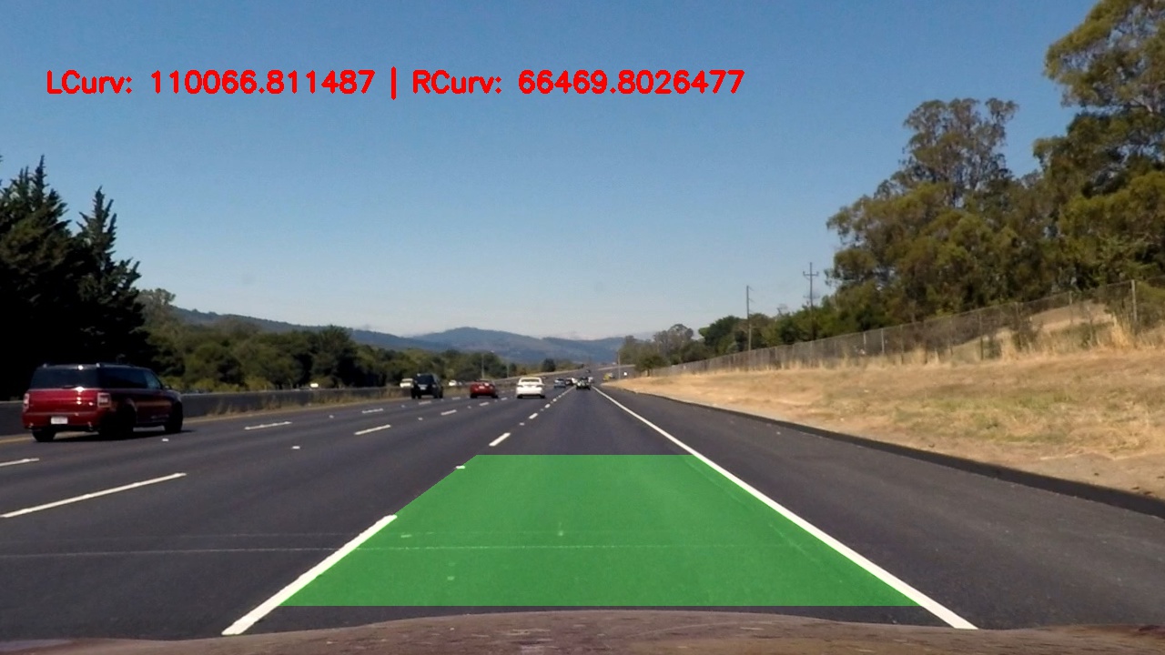
####6. Provide an example image of your result plotted back down onto the road such that the lane area is identified clearly.
Here is an example of my result on a test image:
###Pipeline (video)
####1. Provide a link to your final video output. Your pipeline should perform reasonably well on the entire project video (wobbly lines are ok but no catastrophic failures that would cause the car to drive off the road!).
Here's a link to my video result
###Discussion
####1. Briefly discuss any problems / issues you faced in your implementation of this project. Where will your pipeline likely fail? What could you do to make it more robust?
The approach I took is in itself pretty straight forward. It works well for straight roads or roads with low curvatures but fails in other cases (especially harder_challenge_video). There is many improvement I see possible:
###Adaptive region of interest: in the example of the harder_challenge_video, the position of the car relative to the lanes changes a lot. This requires an approach that can update the patch that will be warped from the image at each frame. This can be done by taking the lane detection from the previous frame and recompute the region of interest such that the lanes end up centered in that roi as much as possible.
###More robust filtering: I noticed that dirt or black spots on the street can really affect the accuracy of the lane detection. The combination of filters I came up with doesn't seem to cope well with strong brightness fluctuations as well. Further work can be done here too. Using HSV targeted at extracting yellow and white colors could be a good approach (I did that in the first project)
