graphlayouts

The name of the package has changed from smglr to graphlayouts.

(When I started this package, my intention was to only implement stress majorization for graph layouts. However, over time, I added some more algorithms so that the former name does not really make sense anymore. Also, this change hopefully gives me an incentive to further extend the package.)

The package implements some graph layout algorithms that are not available in igraph. See my blog post for an introduction on stress majorization.

So far, the package implements four algorithms:

Stress majorization (Paper)
Quadrilateral backbone layout (Paper)
flexible radial layouts (Paper)
spectral layouts

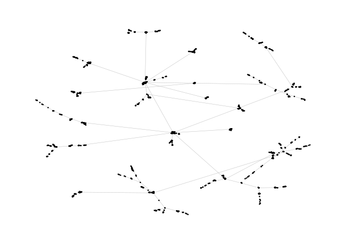
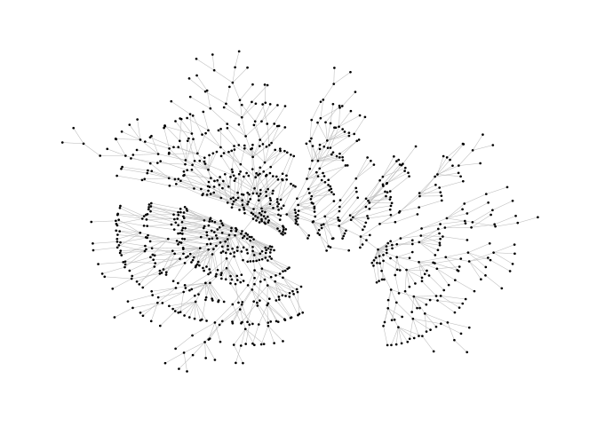
Stress Majorization: Connected Network

This example is a bit of a special case since it exploits some weird issues in igraph.

library(igraph)   
library(ggraph)   
# devtools::install_github("schochastics/graphlayouts")
library(graphlayouts)

set.seed(666)
pa <- sample_pa(1000,1,1,directed = F)

ggraph(pa)+
  geom_edge_link(width=0.2,colour="grey")+
  geom_node_point(col="black",size=0.3)+
  theme_graph()

ggraph(pa,layout="stress")+
  geom_edge_link(width=0.2,colour="grey")+
  geom_node_point(col="black",size=0.3)+
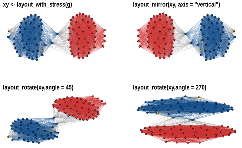
  theme_graph()

Layout manipulation

The functions layout_mirror() and layout_rotate() can be used to manipulate an existing layout

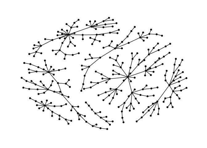
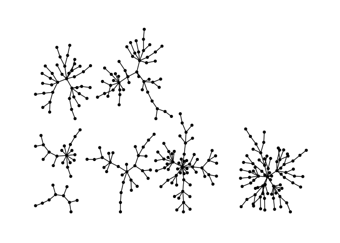
Stress Majorization: Unconnected Network

Stress majorization also works for networks with several components. It relies on a bin packing algorithm to efficiently put the components in a rectangle, rather than a circle.

set.seed(666)
g <- disjoint_union(
  sample_pa(10,directed = F),
  sample_pa(20,directed = F),
  sample_pa(30,directed = F),
  sample_pa(40,directed = F),
  sample_pa(50,directed = F),
  sample_pa(60,directed = F),
  sample_pa(80,directed = F)
)

ggraph(g) +
  geom_edge_link() +
  geom_node_point() +
  theme_graph()

ggraph(g, layout="stress") +
  geom_edge_link() +
  geom_node_point() +
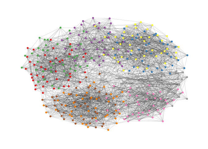
  theme_graph()

Backbone Layout

Backbone layouts are helpful for drawing hairballs.

set.seed(665)
#create network with a group structure
g <- sample_islands(9,40,0.4,15)
g <- simplify(g)
V(g)$grp <- as.character(rep(1:9,each=40))

ggraph(g,layout="stress")+
  geom_edge_link(colour=rgb(0,0,0,0.5),width=0.1)+
  geom_node_point(aes(col=grp))+
  scale_color_brewer(palette = "Set1")+
  theme_graph()+
  theme(legend.position = "none")

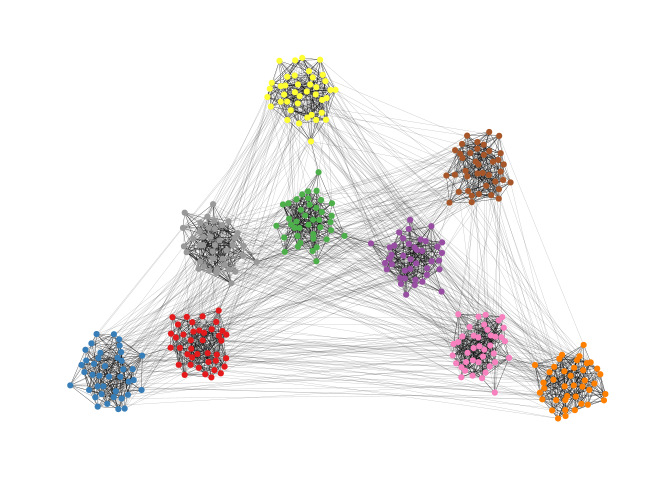
The backbone layout helps to uncover potential group structures based on edge embeddedness and puts more emphasis on this structure in the layout.

bb <- layout_as_backbone(g,keep=0.4)
E(g)$col <- F
E(g)$col[bb$backbone] <- T

ggraph(g,layout="manual",node.positions=data.frame(x=bb$xy[,1],y=bb$xy[,2]))+
  geom_edge_link(aes(col=col),width=0.1)+
  geom_node_point(aes(col=grp))+
  scale_color_brewer(palette = "Set1")+
  scale_edge_color_manual(values=c(rgb(0,0,0,0.3),rgb(0,0,0,1)))+
  theme_graph()+
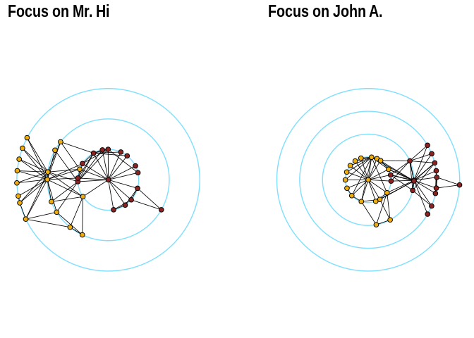
  theme(legend.position = "none")

Radial Layout with Focal Node

The function layout_with_focus creates a radial layout around a focal node. All nodes with the same distance from the focal node are on the same circle.

library(igraphdata)
library(patchwork)
data("karate")

p1 <- ggraph(karate,layout = "focus",v = 1) +
  draw_circle(use = "focus",max.circle = 3)+
  geom_edge_link(edge_color="black",edge_width=0.3)+
  geom_node_point(aes(fill=as.factor(Faction)),size=2,shape=21)+
  scale_fill_manual(values=c("#8B2323", "#EEAD0E"))+
  theme_graph()+
  theme(legend.position = "none")+
  coord_fixed()+
  labs(title= "Focus on Mr. Hi")

p2 <- ggraph(karate,layout = "focus",v = 34) +
  draw_circle(use = "focus",max.circle = 4)+
  geom_edge_link(edge_color="black",edge_width=0.3)+
  geom_node_point(aes(fill=as.factor(Faction)),size=2,shape=21)+
  scale_fill_manual(values=c("#8B2323", "#EEAD0E"))+
  theme_graph()+
  theme(legend.position = "none")+
  coord_fixed()+
  labs(title= "Focus on John A.")

p1+p2

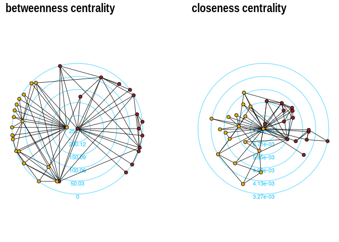
Radial Centrality Layout

The function layout_with_centrality creates a radial layout around the node with the highest centrality value. The further outside a node is, the more peripheral it is.

bc <- betweenness(karate)
p1 <- ggraph(karate,layout = "centrality", cent = bc, tseq = seq(0,1,0.15)) +
  draw_circle(use = "cent") +
  annotate_circle(bc,format="",pos="bottom") +
  geom_edge_link(edge_color="black",edge_width=0.3)+
  geom_node_point(aes(fill=as.factor(Faction)),size=2,shape=21)+
  scale_fill_manual(values=c("#8B2323", "#EEAD0E"))+
  theme_graph()+
  theme(legend.position = "none")+
  coord_fixed()+
  labs(title="betweenness centrality")


cc <- closeness(karate)
p2 <- ggraph(karate,layout = "centrality", cent = cc, tseq = seq(0,1,0.2)) +
  draw_circle(use = "cent") +
  annotate_circle(cc,format="scientific",pos="bottom") +
  geom_edge_link(edge_color="black",edge_width=0.3)+
  geom_node_point(aes(fill=as.factor(Faction)),size=2,shape=21)+
  scale_fill_manual(values=c("#8B2323", "#EEAD0E"))+
  theme_graph()+
  theme(legend.position = "none")+
  coord_fixed()+
  labs(title="closeness centrality")

p1+p2

mbojan / graphlayouts