Example simulations using WaterLily.jl
This repository contains example simulations using the WaterLily.jl package. Some tutorials are presented as Pluto.jl notebooks and the rest are Julia scripts. The examples are divided into 2D and 3D simulations and are listed below. The examples are intended to demonstrate the capabilities of the WaterLily.jl package and to provide a starting point for users to create their own simulations.
An excellent initial tutorial on how to use WaterLily is available on youtube, it will help you go through the basics of the package and how to set up a simple simulation
Two example notebooks are available to help you get started with WaterLily, they are available in the notebooks folder, have a look here if you don't know how to use Pluto.

Below we provide a list of all the examples available
- 2D flow around a circle
- 2D flow around a circle with periodic boundary conditions
- 2D flow around a circle in 1DOF vortex-induced-vibration
- 2D flow around a flapping plate
- 2D flow around the Julia logo
- 2D Lid-driven cavity flow (show how to overwrite BC! function)
- 2D flow around multiple cylinders using the AutoBodies
- 2D flow around a circle with oscillating body force
- 2D flow around circle in an accelerating frame of reference using time-dependent boundary conditions
- 2D flow around a square using AutoBodies set operations
- 2D Tandem airfoil motion optimisation using AutoDiff
- 2D flow around a triangle with a custom sdf
- 2D flow around a circle fully in the terminal
- 2D channel flow with periodic BCs
- 3D Taylor-Green vortex break down
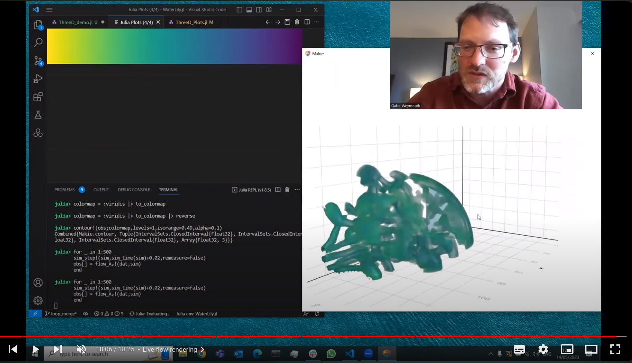
- 3D donut flow, using the GPU and Makie for live rendering
- 3D jellyfish, using the GPU and Makie for live rendering
- 3D cylinder flow with vtk file save ad restart
We define the size of the simulation domain as nm cells. The circle has radius m/8 and is centered at (m/2,m/2). The flow boundary conditions are (U,0), where we set U=1, and the Reynolds number is Re=U*radius/ν where ν (Greek "nu" U+03BD, not Latin lowercase "v") is the kinematic viscosity of the fluid.
using WaterLily
function circle(n,m;Re=250,U=1)
    radius, center = m/8, m/2
    body = AutoBody((x,t)->√sum(abs2, x .- center) - radius)
    Simulation((n,m), (U,0), radius; ν=U*radius/Re, body)
end
The second to last line defines the circle geometry using a signed distance function. The AutoBody function uses automatic differentiation to infer the other geometric parameter automatically. Replace the circle's distance function with any other, and now you have the flow around something else... such as a donut or the Julia logo. Finally, the last line defines the Simulation by passing in parameters we've defined.
Now we can create a simulation (first line) and run it forward in time (third line)
circ = circle(3*2^6,2^7)
t_end = 10
sim_step!(circ,t_end)
Note we've set n,m to be multiples of powers of 2, which is important when using the (very fast) geometric multi-grid solver. We can now access and plot whatever variables we like. For example, we could print the velocity at I::CartesianIndex using println(circ.flow.u[I]) or plot the whole pressure field using
using Plots
contour(circ.flow.p')
A set of flow metric functions have been implemented and the examples use these to make gifs such as the one above.
The three-dimensional Taylor Green Vortex demonstrates many of the other available simulation options. First, you can simulate a non-trivial initial velocity field by passing in a vector function uλ(i,xyz) where i ∈ (1,2,3) indicates the velocity component uᵢ and xyz=[x,y,z] is the position vector.
function TGV(; pow=6, Re=1e5, T=Float64, mem=Array)
    # Define vortex size, velocity, viscosity
    L = 2^pow; U = 1; ν = U*L/Re
    # Taylor-Green-Vortex initial velocity field
    function uλ(i,xyz)
        x,y,z = @. (xyz-1.5)*π/L               # scaled coordinates
        i==1 && return -U*sin(x)*cos(y)*cos(z) # u_x
        i==2 && return  U*cos(x)*sin(y)*cos(z) # u_y
        return 0.                              # u_z
    end
    # Initialize simulation
    return Simulation((L, L, L), (0, 0, 0), L; U, uλ, ν, T, mem)
end
This example also demonstrates the floating point type (T=Float64) and array memory type (mem=Array) options. For example, to run on an NVIDIA GPU we only need to import the CUDA.jl library and initialize the Simulation memory on that device.
import CUDA
@assert CUDA.functional()
vortex = TGV(T=Float32,mem=CUDA.CuArray)
sim_step!(vortex,1)
For an AMD GPU, use import AMDGPU and mem=AMDGPU.ROCArray. Note that Julia 1.9 is required for AMD GPUs.

You can simulate moving bodies in WaterLily by passing a coordinate map to AutoBody in addition to the sdf.
using StaticArrays
function hover(L=2^5;Re=250,U=1,amp=π/4,ϵ=0.5,thk=2ϵ+√2)
    # Line segment SDF
    function sdf(x,t)
        y = x .- SA[0,clamp(x[2],-L/2,L/2)]
        √sum(abs2,y)-thk/2
    end
    # Oscillating motion and rotation
    function map(x,t)
        α = amp*cos(t*U/L); R = SA[cos(α) sin(α); -sin(α) cos(α)]
        R * (x - SA[3L-L*sin(t*U/L),4L])
    end
    Simulation((6L,6L),(0,0),L;U,ν=U*L/Re,body=AutoBody(sdf,map),ϵ)
end
In this example, the sdf function defines a line segment from -L/2 ≤ x[2] ≤ L/2 with a thickness thk. To make the line segment move, we define a coordinate transformation function map(x,t). In this example, the coordinate x is shifted by (3L,4L) at time t=0, which moves the center of the segment to this point. However, the horizontal shift varies harmonically in time, sweeping the segment left and right during the simulation. The example also rotates the segment using the rotation matrix R = [cos(α) sin(α); -sin(α) cos(α)] where the angle α is also varied harmonically. The combined result is a thin flapping line, similar to a cross-section of a hovering insect wing.
One important thing to note here is the use of StaticArrays to define the sdf and map. This speeds up the simulation since it eliminates allocations at every grid cell and time step.

This example demonstrates a 2D oscillating periodic flow over a circle.
function circle(n,m;Re=250,U=1)
    # define a circle at the domain center
    radius = m/8
    body = AutoBody((x,t)->√sum(abs2, x .- (n/2,m/2)) - radius)

    # define time-varying body force `g` and periodic direction `perdir`
    accelScale, timeScale = U^2/2radius, radius/U
    g(i,t) = i==1 ? -2accelScale*sin(t/timeScale) : 0
    Simulation((n,m), (U,0), radius; ν=U*radius/Re, body, g, perdir=(1,))
end
The g argument accepts a function with direction (i) and time (t) arguments. This allows you to create a spatially uniform body force with variations over time. In this example, the function adds a sinusoidal force in the "x" direction i=1, and nothing to the other directions.
The perdir argument is a tuple that specifies the directions to which periodic boundary conditions should be applied. Any number of directions may be defined as periodic, but in this example only the i=1 direction is used allowing the flow to accelerate freely in this direction.
WaterLily gives the possibility to set up a Simulation using time-varying boundary conditions for the velocity field, as demonstrated in this example. This can be used to simulate a flow in an accelerating reference frame. The following example demonstrates how to set up a Simulation with a time-varying velocity field.
using WaterLily
# define time-varying velocity boundary conditions
Ut(i,t::T;a0=0.5) where T = i==1 ? convert(T, a0*t) : zero(T)
# pass that to the function that creates the simulation
sim = Simulation((256,256), Ut, 32)
The Ut function is used to define the time-varying velocity field. In this example, the velocity in the "x" direction is set to a0*t where a0 is the acceleration of the reference frame. The Simulation function is then called with the Ut function as the second argument. The simulation will then run with the time-varying velocity field.
In addition to the standard free-slip (or reflective) boundary conditions, WaterLily also supports periodic boundary conditions, as demonstrated in this example. For instance, to set up a Simulation with periodic boundary conditions in the "y" direction the perdir=(2,) keyword argument should be passed
using WaterLily,StaticArrays

# sdf an map for a moving circle in y-direction
function sdf(x,t)
    norm2(SA[x[1]-192,mod(x[2]-384,384)-192])-32
end
function map(x,t)
    x.-SA[0.,t/2]
end

# make a body
body = AutoBody(sdf, map)

# y-periodic boundary conditions
Simulation((512,384), (1,0), 32; body, perdir=(2,))
Additionally, the flag exitBC=true can be passed to the Simulation function to enable convective boundary conditions. This will apply a 1D convective exit in the x direction (currently, only the x direction is supported for the convective outlet BC). The exitBC flag is set to false by default. In this case, the boundary condition is set to the corresponding value of the u_BC vector specified when constructing the Simulation.
using WaterLily

# make a body
body = AutoBody(sdf, map)

# y-periodic boundary conditions
Simulation((512,384), u_BC=(1,0), L=32; body, exitBC=true)The following example demonstrates how to write simulation data to a .pvd file using the WriteVTK package and the WaterLily vtkwriter function. The simplest writer can be instantiated with
using WaterLily,WriteVTK

# make a sim
sim = make_sim(...)

# make a writer
writer = vtkwriter("simple_writer")

# write the data
write!(writer,sim)

# don't forget to close the file
close(writer)
This would write the velocity and pressure fields to a file named simmple_writer.pvd. The vtkwriter function can also take a dictionary of custom attributes to write to the file. For example, the following code can be run to write the body signed-distance function and λ₂ fields to the file
using WaterLily,WriteVTK

# make a writer with some attributes, need to output to CPU array to save file (|> Array)
velocity(a::Simulation) = a.flow.u |> Array;
pressure(a::Simulation) = a.flow.p |> Array;
_body(a::Simulation) = (measure_sdf!(a.flow.σ, a.body, WaterLily.time(a));
                                     a.flow.σ |> Array;)
lamda(a::Simulation) = (@inside a.flow.σ[I] = WaterLily.λ₂(I, a.flow.u);
                        a.flow.σ |> Array;)

# map field names to values in the file
custom_attrib = Dict(
    "Velocity" => velocity,
    "Pressure" => pressure,
    "Body" => _body,
    "Lambda" => lamda
)

# make the writer
writer = vtkWriter("advanced_writer"; attrib=custom_attrib)
...
close(writer)
The functions that are passed to the attrib (custom attributes) must follow the same structure as what is shown in this example, that is, given a Simulation, return an N-dimensional (scalar or vector) field. The vtkwriter function will automatically write the data to a .pvd file, which can be read by ParaView. The prototype for the vtkwriter function is:
# prototype vtk writer function
custom_vtk_function(a::Simulation) = ... |> Array
where ... should be replaced with the code that generates the field you want to write to the file. The piping to a (CPU) Array is necessary to ensure that the data is written to the CPU before being written to the file for GPU simulations.
The restart of a simulation from a VTK file is demonstrated in this example. The ReadVTK package is used to read simulation data from a .pvd file. This .pvd must have been written with the vtkwriter function and must contain at least the velocity and pressure fields. The following example demonstrates how to restart a simulation from a .pvd file using the ReadVTK package and the WaterLily vtkreader function
using WaterLily,ReadVTK
sim = make_sim(...)
# restart the simulation
writer = restart_sim!(sim; fname="file_restart.pvd")

# append sim data to the file used for restart
write!(writer, sim)

# don't forget to close the file
close(writer)
Internally, this function reads the last file in the .pvd file and use that to set the velocity and pressure fields in the simulation. The sim_time is also set to the last value saved in the .pvd file. The function also returns a vtkwriter that will append the new data to the file used to restart the simulation. Note that the simulation object sim that will be filled must be identical to the one saved to the file for this restart to work, that is, the same size, same body, etc.
Sometime, it might be usefull to overwrite the default functions used in the simulation. For example, the BC! function can be overwritten to implement a custom boundary condition, see this example. For example to overwrite the mom_step! function you will need something like this
function WaterLily.mom_step!(a::Flow{N},b::AbstractPoisson) where N
    ...do your thing...
end
in your main script. This means that internally, when EaterLily call mom_step! it will call this ew function and not the one in src/Flow.jl. This can be used to implement custom boundary conditions, custom body forces, etc.
NOTE: In WaterLily we use a staggered grid, this means that the velocity component and the pressure are not at the same physical location in the finite-volume mesh, see figure below. You have to be careful if you play with the
BC!function to make sure that you are applying the boundary condition to the correct physical location.

If you have used WaterLily.jl for research, please cite us! The following manuscript describes the main features of the solver and provides benchmarking, validation, and profiling results.
@misc{WeymouthFont2024,
    title         = {WaterLily.jl: A differentiable and backend-agnostic Julia solver to simulate incompressible viscous flow and dynamic bodies},
    author        = {Gabriel D. Weymouth and Bernat Font},
    url           = {https://arxiv.org/abs/2407.16032},
    eprint        = {2407.16032},
    archivePrefix = {arXiv},
    year          = {2024},
    primaryClass  = {physics.flu-dyn}
}
We are always looking for new examples to showcase the capabilities of WaterLily.jl. If you came up with amazing examples and you want to share them, please open a pull request with the new exmaple either as a Pluto.jl notebook or a classic script. We will be happy to review it and merge it into the repository.