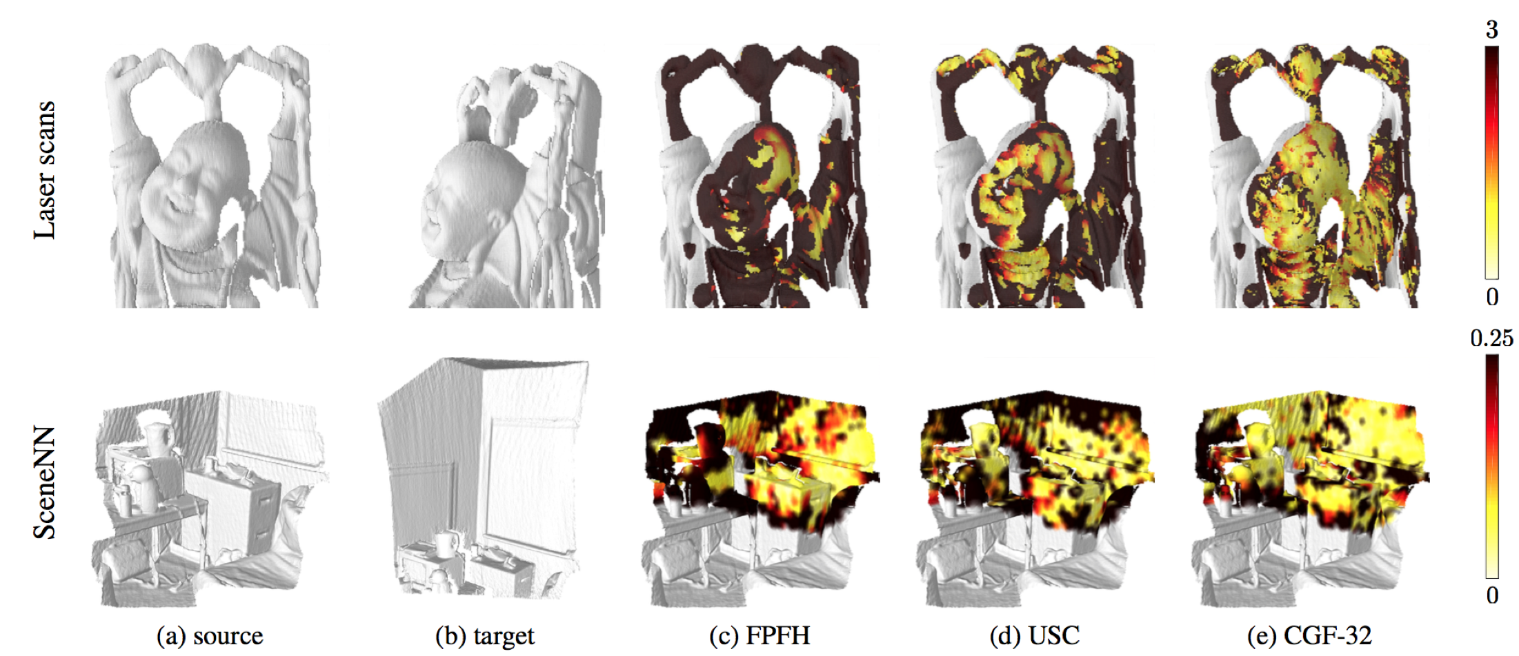
This repository describes the code and dataset used in Learning Compact Geometric Features (ICCV 2017).
Code for computing geometric features using our pretrained models is included in the src directory. The code has dependencies on the Point Cloud Library (PCL), the compression library LZF, and optionally OpenMP. We've included the LZF library in the src directory in the folder liblzf-3.6. PCL can be installed using brew -- brew install pcl -- or from source.
The pipeline to generate features from point cloud data consists of three files.
main.cpp: Computes the raw spherical histograms from a point cloud with normals provided in the PCD format.compress.py: Converts from the compressed LZF representation to a compressed numpy file.embedding.py: Computes geometric features using a pretrained model. Can also be used to train new models.
We have provided a cmake file to compile main.cpp for convenience. Simply run the following commands in the src directory.
cmake .
make
This will create an executable main which has the following options.
Usage: ./main [options] <input.pcd>

Options:
--relative If selected, scale is relative to the diameter of the model (-d). Otherwise scale is absolute.
-r R Number of subdivisions in the radial direction. Default 17.
-p P Number of subdivisions in the elevation direction. Default 11.
-a A Number of subdivisions in the azimuth direction. Default 12.
-s S Radius of sphere around each point. Default 1.18 (absolute) or 17% of diameter (relative).
-d D Diameter of full model. Must be provided for relative scale.
-m M Smallest radial subdivision. Default 0.1 (absolute) or 1.5% of diameter (relative).
-l L Search radius for local reference frame. Default 0.25 (absolute) or 2% of diameter (relative).
-t T Number of threads. Default 16.
-o Output file name.
-h Help menu.
The program has two possible settings for the scale: relative and absolute. The relative setting sets the search radius, the local reference frame radius, and the minimal radial subdivision in terms of percentages of the diameter of the model. In this case the diameter of the model must also be given. The absolute setting simply uses the provided values, assuming the units are in meters. The default values are the same as those used in the paper. Models trained on laser scan data were provided inputs defined using relative scale, while SceneNN models used absolute scale.
The provided models are trained for the default values. Thus when using our pretrained models it is best to use the default settings for the spherical histograms. However the radial, elevation, and azimuth subdivions can be specified, which would require training a new model for the new parameterization. Typical usage will look something like the following.
./main -d 10 -s 1.7 -l 0.2 input.pcd
./main --relative -d 10 input.pcd
Attempt to keep the search radius around 17% of the diameter, as that is what the models are trained on. Slight deviation from this value may improve results in some cases.
It is of the utmost importance that the input point cloud contain oriented normals that are consistently oriented across all point clouds to be matched. In our experiments we oriented the normals to the location of the camera, but any consistent orientation will do.
The result of running main is a file containing the raw spherical histograms compressed using the LZF algorithm. The following command converts this representation to a compressed numpy file.
python compress.py output.lzf 2244 output.npz
The value 2244 is the feature length and is equal to the number of bins in the spherical histogram. The defaults in the paper are 17 radial subdivision, 11 elevation subdivisions, and 12 azimuth subdivisions, giving a feature length of 2244.
Once our data is in this format we can run the following command to compute our learned geometric features.
python embedding.py --evaluate=True --checkpoint_model=/path/to/pretrainedmodel.ckpt --output_file=learned_features.npz input.npz
This command loads the specified pretrained model and evalutes the embedding on the input feautures in input.npz. See the top of embedding.py for default values for each of these fields.
We can also train a new model using embedding.py by running a command similar to the following.
python embedding.py --evaluate=False --summaries_dir=./summaries/ --checkpoint_dir=./checkpoints/ --max_steps==1000000 input.npz
To train a new model the input.npz need only contain the raw spherical histograms in a field called data and the triplets for the embedding loss in a field called triplets. See the provided SceneNN dataset for more details.
Lastly for further speed improvements the code can be compiled with OpenMP. Simply uncomment the following lines in main.cpp.
//#ifdef _OPENMP
//#pragma omp parallel for num_threads(num_threads)
//#endifThe trained models can be downloaded here.
This zip archive contains a 18 folders each containing a pretrained model trained on either laser scan data or SceneNN. Each folder is named either laserscan_XD or scenenn_XD where X denotes the dimensionality of the output feature.
The dataset is available here.
If you use these features in your own research, please cite the following paper.
Marc Khoury, Qian-Yi Zhou, and Vladlen Koltun. Learning Compact Geometric Features. ICCV 2017. Bibtex
