Distributed Graph Algorithms

This is an archive of some of the work I did in a class on distributed algorithms I took at Stony Brook University. The class was a rare one-time undergrature offering of a normally graduate course. The instructor at the time was Annie Liu. It is offered these days as CSE 535 Asynchronous Systems.

This repository contains the implementations of certain distributed graph algorithms in a language known as DistAlgo. DistAlgo is a superset of Python that adds special constructs to Python for specifying distributed algorithms in a high-level and succint manner. DistAlgo programs get compiled to portable Python 3 code. DistAlgo was developed at the Department of Computer Science in Stony Brook University.

The Distributed Graph Algorithms

Each of the above algorithms have been documented with thorough description of their algorithms as well as with specific information about their implementations, limitations, etc. They can be found in relevant sections of this ReadMe as well as in the ReadMe containing the algorithms themselves.

The version of DistAlgo used in the implementation of the above algorithms is DistAlgo-0.2. Note: All references have been hyperlinked in-place using Markdown's link syntax.

Dependencies

NetworkX

A graph library known as NetworkX was used in this project. It is a well-renown pure Python library that provides several useful features pertaining to graphs. Granted, it was a bit unnecessary for this project, but I was anticipating more use for it than was needed.

matplotlib

The widely-known library matplotlib is being used here to visualize the various graphs (solutions, inputs, etc.) in this project.

The file tools.py used by the MST solver does stuff like building the NetworkX graph, visualizing it with matplotlib, etc.

Other

Random Graph Generator

In addition, I wrote a simple random graph generator (contained in graph_gen.py) that builds a weighted undirected graph with a user-selected number of ranom randomly-weighed edges between the nodes. It can be executed independently as a script (in addition to being imported and used as a library) as shown below:

    usage: graph_gen.py [-h] [-n NODES] [-e EDGES] [file_name]

    Generate a random graph.

    positional arguments:
      file_name             File to write the graph to, listing the edges of a
                            graph line-by-line in the following style: "A B 2",
                            where "A" and "B" are node names and "2" is the weight
                            of the edge connecting them.

    optional arguments:
      -h, --help            show this help message and exit
      -n NODES, --nodes NODES
                            The maximum number of nodes in the graph.
      -e EDGES, --edges EDGES
                            The number of edges in the graph.

Token-based Distributed Mutex Algorithms

Ricart-Agrawala's and Suzuki-Kasami's token-based distributed mutex algorithms have also been been implemented in DistAlgo-0.2. In addition, Lamport's fast mutual exclusion and bakery algorithms have been implemented using the built-in Python library threading.

Distributed Minimum Spanning Tree

Overview

This is a distributed program that implements a distributed Minimum Spanning Tree solver in DistAlgo.

Problem Description

A spanning tree is defined as a tree which is a sub-graph of a given graph and connects all the nodes in the graph. The graph must be a connected and undirected graph. A Minimum Spanning Tree is a spanning tree whose sum of weights of the edges is the lowest of all possible spanning trees for the given graph.

Same graph, multiple minimum spanning trees

If a graph has multiple edges with the same weight, then the graph could have several MSTs. This situation can be obviated by constructing a graph whose edges have unique weights.

Algorithms

Sequential Solvers

There are two commonly used algorithms for finding the MST of a graph sequentially: Prim's algorithm and Kruskal's algorithm. To better understand the problem and get a feel for it, I wrote a Kruskal's solver which can found at Kruskal.py.

Distributed Solvers

Here the nodes of the graph are nodes in a distributed system; i.e. a set of computers/processes where each computer represents a node of the graph and the edge between two nodes of the graph respresent a communication interlink between two processes. Nodes (processes) without edges between are not allowed to communicate with each other.

The best known algorithm that solves this problem is the GHS algorithm of R. G. Gallager, P. A. Humblet and P. M. Spira. According to Wikipedia, there also is a parallelization of Prim's sequential algorithm by Nobri et al. The GHS algorithm could be considered the state of art for the distributed MST problem. I have implemented the GHS algorithm using DistAlgo, a superset of Python enhanced for distributed programming by Annie Liu, Bo Lin et al. from Stony Brook University.

A pre-condition for the GHS aglorithm is that the MST be unique, i.e. that all edges have unique weights.

Papers on GHS

I found two papers online that describe GHS. One is the original from 1983, by Gallager, Humlbet & Spira. The other is an enhanced version of the original (with better graphics, typesetting, explanation, etc.) prepared by Guy Flysher and Amir Rubinshtein. I followed the second one while creating my implementation in DistAlgo.

I've posted PDFs of both papers (found online) in this GitHub repo under the papers directory. Links to them are below:

The Original paper by Gallager, Humblet and Spira from 1983.
The enhanced version of the original prepared by Guy Flysher and Amir Rubinshtein. (I recommend this one)

High-level Explanation of the GHS Algorithm

The algorithm hinges on the idea of a "fragment of the MST". It relies on this property of MSTs:

If F is a fragment of an MST M, then joining the node of the other end of the minimum weight "outgoing" edge will yield yet another fragment of M. Here, "outgoing" is defined as an edge which connects (any node in) the fragment to a node that is not part of the fragment.

The algorithm initially starts out by assigning each node to a fragment of its own. It then proceeds to to follow a set of steps to merge the fragments over and over again, until there is only one fragment left. The final fragment is equal to the MST for the graph. Additionally, each fragment has a property called its level which determines what kind of merge process occurs between two fragments. There are two kinds of merges: absorptions and level-augmenting merges.

The steps followed by the aglorithm are:

Initially, all fragments are at level 0 and contain just the one node. Additionally, all nodes are sleeping at first.
A node has to be woken up before it can do anything. A nicety of the GHS algorithm is that there are no restriction whatsoever on the wakeup process. One may opt, if necessary, to wake up all nodes immediately; or alternatively wake up just one single node. In the course of the algorithm, all nodes will eventually be owken up. Other operations in the algorithm result in other nodes waking up.
Every fragment finds its minimum weight outgoing edge and sends a Connect request over it containing the level of the fragment it belongs to.
Every time a fragment sends a Connect to another fragment, it enters a "waiting" state (denoted by FOUND in the code.) The fragment then, waits until is either gets absorbed by or merges with the other fragment.
When a fragment receives a Connect, the conditions that determine whether it should absorb or merge with the requesting fragment are as follows:
- If the fragment it received the Connect request from is of a lower level, then that fragment gets absorbed immediately.
- If the fragment it received the Connect request from is of a level equal to its own or higher, two things can happen:
  - If the fragment receving the Connect has also sent a Connect to the other fragment, they merge.
  - In any other case, the fragment simply does not reply and waits for the situation to change. The way the algorithm works, a merge or absorption will occur eventually.
The termination case for the algorithm is, when a fragment is unable to find a minimum weight outgoing edge. This case means that it is the only fragment left. Therefore it must be the complete MST.
Finally two important thing to note are:
- Fragments of level-1 and above, are controlled by a pair of nodes called the core nodes. These nodes are first formed during the initial level-0 Connect exchanges. Nodes sending _Connect_s to each other form a level-1 fragment.
- Fragments are identified by the weight of the edge between the core nodes. Since, all edges have to be unique as pre-requisite for the GHS algorithm, the edge weight can be used to uniquely identify a fragment.

There is a lot more to inner working of the algorithms, such as how exactly mergers and absorptions occur, how the minimum weight outgoing edge is found, etc. However these details would be too low-level to be discussed in this document.

The following diagram (from Guy Flysher and Amir Rubinshtein's version of the GHS paper) illustrates the fragment absorption and merge processes:

Pseudocode

The pseudocode for GHS provided in the paper is quite low-level. I tried, but wasn't able to directly translate it to DistAlgo. The main problem I ran into it was that, DistAlgo does not provide a way (or I don't know of a way) to manipulate the local message queue directly. The pseudocode uses that ability to "delay" processing a message, by putting it back in the end of the queue. My implementation differs in this aspect and also other aspects that make it more high-level and easier to understand (but less efficient.)

I largely followed the pseudocode as a guide, rather than following it directly. For my implementation I tried, to the maximal extent possible, to work out the lower level details myself, while simply following the high-level details of the algirithm as described and shown in the diagram above. The benefit of following the high-level explanation was that, I was able to keep the big picture in my head (all at once.) I found that impossible to do with the pseudocode (or with the low-level description, which contains a lot of minute details that are intricately connected with each other.) I found I was able to understand part of it at a time, but to hold the whole thing in my head at once was impossible.

The following is an image of the pseudocode for GHS extracted from Guy Flysher and Amir Rubinshtein's version of the paper:

Implementation

The implementation is in DistAlgo 0.2. There are two algorithms: Kruskal's in Kruskal.py and GHS in MST.dis.py. I wrote Kruskal's just an exercise early on to get a better understanding of MSTs (and in an attempt to come up with my own distirbuted algorithm.) The relevant program in contained in its entirety in the file MST.dis.py in this directory. The .py was added to obtain syntax highlighting in GitHub. It is pointed to by the symlink MST.dis. MST.dis can be run using DistAlgo by typing: python3 -m distalgo.runtime MST.dis. Alternatively, there's a script run.py which does the same thing.

Usage

Both the GHS algorithm (in MST.dis.py) and Kruskal.py import the module tools.py which provides a common set of services like handling optargs, constructing the graph from a graph file and visualizing the solution using matplotlib. The graph file is a simple text file which lists all the edges in the graph in CSV-style, except without the commas. If no graph file is passed, then graph-2 is used by default. tools.py builds from the graph file, a NetworkX graph object representing it.

The available arguments and purposes can be displayed by passing the -h argument to display the help message:

usage: MST.dis [-h] [-v] [-b BACKEND] [-o OUTPUT] [graph]

Finds the Minimum Spanning Tree (MST) of a given graph.

positional arguments:
  graph                 File listing the edges of a graph line-by-line in the
                        following style: "A B 2", where "A" and "B" are node
                        names and "2" is the weight of the edge connecting
                        them.

optional arguments:
  -h, --help            show this help message and exit
  -v, --visualize       Visualize the graph and its solution using matplotlib,
                        with the branches of the MST marked in thick blue.
  -b BACKEND, --backend BACKEND
                        Interactive GUI backend to be used by matplotlib for
                        visualization. Potential options are: GTK, GTKAgg,
                        GTKCairo, FltkAgg, MacOSX, QtAgg, Qt4Agg, TkAgg, WX,
                        WXAgg, CocoaAgg, GTK3Cairo, GTK3Agg. Default value is
                        Qt4Agg.
  -o OUTPUT, --output OUTPUT
                        File to write the solution (MST edge list) to. By
                        default it written to the file `sol`.

The Spark process

The Spark process is another process that is present in my implementation in addition to the node processes. It's job solely bureaucratic: to start the algorithm by waking up atleast one node, and to finish up the algorithm and present the results.

It accomplishes starting the algorithm by simply picking a node at random and sending it a Wakeup message. As an interesting side note, the GHS algorithm allows any number of nodes to be woken up spontaneously. This aspect of the GHS algorithm can be easily tested by un-commenting two lines of code in Spark's main() function. The two lines send Wakeup messages to all nodes rather one random node.

Finally, output collection starts after Spark receives a Finished message from one of the two core nodes. Subsequently, it sends a QueryBranches message to every node process, and they all reply with the edges they know to be branches. (No single node knows all the branches of the MST, only which of its edges are branches.) The Spark processes collects these results and combines them in a set, then outputs the solution using DistAlgo, and finally passes it on to toos.py to write it down to a file and/or visualize it using matplotlib.

Running

When MST.dis is run (by typing python3 -m distalgo.runtime MST.dis or using run.py), the program produces a long list of output messages, each emenating from the processes representing the nodes describing operations that occured at the node. A truncated example of the output is shown below:

[2012-10-11 17:18:47,434]runtime:INFO: Creating instances of Node..
[2012-10-11 17:18:47,458]runtime:INFO: 13 instances of Node created.
[2012-10-11 17:18:47,464]runtime:INFO: Creating instances of Spark..
[2012-10-11 17:18:47,465]runtime:INFO: 1 instances of Spark created.
[2012-10-11 17:18:47,472]runtime:INFO: Starting procs...
[2012-10-11 17:18:47,473]runtime:INFO: Starting procs...
[2012-10-11 17:18:47,475]Node(F):INFO: Received spontaneous Wakeup from: Spark
[2012-10-11 17:18:47,475]Node(F):INFO: F is waking up!
[2012-10-11 17:18:47,477]Node(E):INFO: Received Connect(0) from: F
[2012-10-11 17:18:47,477]Node(E):INFO: E is waking up!
[2012-10-11 17:18:47,478]Node(F):INFO: Received Connect(0) from: E
[2012-10-11 17:18:47,478]Node(E):INFO: E merging with F
[2012-10-11 17:18:47,479]Node(F):INFO: F merging with E
[2012-10-11 17:18:47,480]Node(F):INFO: Received Initiate(1, 1, 'Find') from: E
[2012-10-11 17:18:47,480]Node(E):INFO: Received Initiate(1, 1, 'Find') from: F
[2012-10-11 17:18:47,481]Node(F):INFO: F has sent Test() to A
[2012-10-11 17:18:47,481]Node(E):INFO: E has sent Test() to H
[2012-10-11 17:18:47,481]Node(A):INFO: Received Test(1, 1) from: F
[2012-10-11 17:18:47,482]Node(A):INFO: A is waking up!
[2012-10-11 17:18:47,482]Node(H):INFO: Received Test(1, 1) from: E
[2012-10-11 17:18:47,482]Node(H):INFO: H is waking up!
...
[2012-10-11 17:18:47,529]Node(M):INFO: M merging with L
[2012-10-11 17:18:47,530]Node(L):INFO: L merging with M
....
[2012-10-11 17:18:47,537]Node(K):INFO: K has sent Test() to J
[2012-10-11 17:18:47,537]Node(J):INFO: Received Test(1, 20) from: K
[2012-10-11 17:18:47,538]Node(J):INFO: J sent Accept() to K
[2012-10-11 17:18:47,538]Node(K):INFO: Outgoing Neighbor K -> J @ 23 [find_count = 0]
[2012-10-11 17:18:47,538]Node(K):INFO: Least weight(23) outgoing edge from K: K -> J
[2012-10-11 17:18:47,539]Node(L):INFO: Received [K, J] @ 23 from K [find_count = 0]
[2012-10-11 17:18:47,539]Node(L):INFO: Least weight(23) outgoing edge from L: L -> K -> J
[2012-10-11 17:18:47,540]Node(L):INFO: Least weight(23) outgoing edge of fragment(20): L -> K -> J !!!!!!!!!!!!!!!
[2012-10-11 17:18:47,540]Node(M):INFO: Received [L, K, J] @ 23 from other core node L
[2012-10-11 17:18:47,541]Node(K):INFO: Fragment (20) ------------ Sending Connect(1) to J
[2012-10-11 17:18:47,541]Node(J):INFO: Received Connect(1) from: K
[2012-10-11 17:18:47,542]Node(J):INFO: J absorbing K
[2012-10-11 17:18:47,542]Node(J):INFO: J has sent FIND to branch K
[2012-10-11 17:18:47,542]Node(K):INFO: Received Initiate(2, 10, 'Find') from: J
[2012-10-11 17:18:47,543]Node(K):INFO: K has sent FIND to branch L
[2012-10-11 17:18:47,543]Node(L):INFO: Received Initiate(2, 10, 'Find') from: K
[2012-10-11 17:18:47,543]Node(L):INFO: L has sent FIND to branch M
[2012-10-11 17:18:47,544]Node(J):INFO: J Received Reject() from: K
[2012-10-11 17:18:47,544]Node(M):INFO: Received Initiate(2, 10, 'Find') from: L
[2012-10-11 17:18:47,544]Node(M):INFO: Least weight(999999999) outgoing edge from M: No Outgoing edges
[2012-10-11 17:18:47,543]Node(K):INFO: K sent Reject() to J
[2012-10-11 17:18:47,545]Node(L):INFO: Received None @ 999999999 from M [find_count = 0]
[2012-10-11 17:18:47,545]Node(L):INFO: Least weight(999999999) outgoing edge from L: No Outgoing edges
[2012-10-11 17:18:47,546]Node(K):INFO: Received None @ 999999999 from L [find_count = 0]
[2012-10-11 17:18:47,546]Node(K):INFO: Least weight(999999999) outgoing edge from K: No Outgoing edges
[2012-10-11 17:18:47,547]Node(J):INFO: Received None @ 999999999 from K [find_count = 0]
[2012-10-11 17:18:47,547]Node(J):INFO: Least weight(999999999) outgoing edge from J: No Outgoing edges
[2012-10-11 17:18:47,548]Node(I):INFO: Received None @ 999999999 from J [find_count = 0]
[2012-10-11 17:18:47,548]Node(I):INFO: Least weight(999999999) outgoing edge from I: No Outgoing edges
[2012-10-11 17:18:47,549]Node(I):INFO: ----- NO MORE OUTGOING EDGES -----
[2012-10-11 17:18:47,549]Node(E):INFO: Received None @ 999999999 from other core node I
[2012-10-11 17:18:47,549]Node(E):INFO: ----- NO MORE OUTGOING EDGES -----
[2012-10-11 17:18:47,575]Spark(Spark):INFO: Solution: (A, B), (A, F), (C, D), (D, I), (E, F), (E, G), (E, H), (E, I), (I, J), (J, K), (K, L), (L, M)
[2012-10-11 17:18:47,592]runtime:INFO: ***** Statistics *****
* Total procs: 14

[2012-10-11 17:18:47,593]runtime:INFO: Terminating...

The 999999999 that can be seen conspicuously towards the end is a constant representing infinity. The "infinite" weight outgoing edge is used to denote the case where there are no outoging edges. When the two core nodes of the final fragment have received replies from all their branches indicating there are no more outoging edges, it sends a message to the special process Spark.

Spark immediately presents the solution, and sends a message to all the nodes indicating the completion of the algorithm. Then the program terminates. Spark presents the solution, by first using DistAlgo's output and printing the solution; and second by drawing the graph using NetworkX and matplotlib if the user has opted to visualize the solution (using the -v option). The visualized graph denotes the branches of the MST using thick blue edges.

Test Cases

The following are a series of test cases run on the algorithm. The main test cases are enclosed in the files: graph-1, graph-2 and graph-3. There is an easy way to verify the solution: Run Kruskal.py against the same graph. Kruskal is quite clever; it verifies its own solution against NetworkX's MST solver so there's no way it could be wrong.

Graph 1

For my initial test case which I used for much of the developed of my algorithm, I wanted to use a graph that was in particular designed to test this algorithm. So I looked online for web pages discussing Minimum Spanning Trees, and I finally came across one that had a graph with all unique weights: http://cgm.cs.mcgill.ca/~hagha/topic28/topic28.html

The following matplotlib diagram was generated representing the solution to graph-1:

The thick blue edges denote the branches of the MST (Minimum Spanning Tree).

What Happens

Some of the key GHS events that occur while solving graph-1 are:

E and F from a Level-1 fragment.
I and J from a Level-1 fragment.
Both level-1 fragments proceed to absorb every other node in the graph.
In the end, these 2 fragments merge across I and E forming a new Level-2 fragment with I and E as the core nodes.

Graph 2

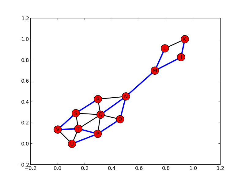
I added three more nodes: L, K and M to the previous graph for increased complexity and to test other aspects of the GHS algortithm. The added steps that occur after adding these three new nodes are:

L, K and M form a Level-1 fragment of their own with L and M as the core nodes.
The L, K and M fragment gets absorbed by the Level-2 fragment with core nodes I and E.

The solution to graph-2 is depicted below:

As always, the thick blue edges denote the branches of the MST.

Graph 3

This is a much more complex test case than the previous ones. I drew a sketch of it on paper:

The edge list for it can be found in the file graph-3. The output produced by MST.dis and Kruskal.py can be found in graph-3-ouptput.txt (in this directory.)

While writing the graph file graph-3, I ran the MST solver several times and obtained these intermediate results:

Intermediate Result 1

Intermediate Result 2

Final Solution

Click to enlarge:

Once again, the blue edges denote the MST.

This third test case tests merges between Level-2 fragments. The final fragment formed at the end of this test case is a Level-3 fragment. The graph-3-ouptput.txt file in this directory shows the output generated by MST.dis while solving this test case.

Random Graph with 100 nodes and 1000 edges

This random graph was generated using the random graph generator (random_graph.py) in the parent directory. A copy of the random graph used for this test case is in the file 1000edge-100node-graph in this directory. The solution diagram, while not helpful per-se, is still shown below:

The output generated by the distributed MST while solving this problem is enclosed in the file 1000edge-100node-graph-output.txt.

Distributed Maximal Independent Set

Overview

Problem Description

This algorithms solves the Maximal independent set problem in a distributed system where the nodes are represented by processes and edges between the nodes in the graph represent a valid communication link between these processes. The maximal independent set problem is described in detail in its Wikipedia article. One of its many applications is graph coloring.

Multiple Maximal Independent Sets for the same graph

For one graph, there can be more than one, and often several maximal independent sets. Most algorithms that solve for maximal independent set involve some random factor, so we can expect different solutions to the MIS problem in different runs of the algorithm.

The following diagram from Wikipedia for the graph of a cube shows the 6 different possible MISs for it:

Best Algorithms

A quick Google search for "distributed maximal independent set" reveals a few algorithms for solving for Maximal Independent Set. The top among these is A Log-Star Distributed Maximal Independent Set Algorithm by Johannes Schneider, Roger Wattenhofer. Another major one that comes up when searching for "parallel maximal independent srt" instead is Luby's algorithm (the original paper and lecture notes on it).

However after looking at these algorithms for a while, I decided to instead design my own solution to the distributed Maximal Independent Set problem. Luby's algorithm for instance, seemed a little more complicated than necessary to me. The complication was probably an optimization for performance. It involves (based on my understanding) picking a random set of vertices, breaking "ties" in the set -- i.e. vertices that formed edges in the random set, and doing something else and repeating the process. In addition, the lecture notes and paper on Luby's algorith, weren't very clear on how the interprocess communication was to be modeled. (In contrast, the GHS paper for MST was very clear about this.) However, it was pretty clear to me what the straightforward parallelization (distribution) of the sequential MIS algorithm would look like, so I decided to design my own distributed algorithm based on it.

Description of the Algorithm

Design

The design of my algorithm largely follows the fundamental idea underpinning the sequential algorithm. The sequential algorithm (taken from these Luby's algorithm lecture notes) for finding MST is shown below:

The core steps in my algorithm are as follows:

Initally all nodes are in a "normal" state. My algorithm, like Luby's involves a random factor. Initially, it picks a random node and marks it as a VERTEX of the MST.
Next, this (randomly-picked) vertex marks all its neighbors as OUT. This means they're not vertices.
The randomly-picked vertex then performs a search for node in the graph, that is neither a VERTEX nor OUT and when it finds, it marks that node as the next VERTEX and repeats the search-and-mark process again.
It repeats this process until is able to find no more NORMAL nodes. At this point it knows the algorithm has ended, and it terminates the program.

Conditions and Constraints

Some of the conditions and constraints placed placed on the algorithm and in the implementatin are:

Each node in the graph is represented by a process.
A process/node can only communicate with other processes/nodes that it has an edge with. This constraint is soft-enforced. Although DistAlgo allows a process to communicate with any other process, the algorithm does not communicate to any process that it does not have an edge with. (An exception is the control process, which is not key player in the algorithm.) This constraint is crucial has been articially imposed upon this algorithm to imiate real-life networks where there necessarily isn't a communication link between every computer with every other computer.
There's a special process known as the Control Process. The Control Process fulfills three roles: (1) It iniates the algorithm. (2) It collects output. (3) It terminates the algorithm.
The control process is not bound by constraint (a), and any process is permitted to communicate to it and it to all other processes. However, the control process isn't absolutely necessary to the algorithm, or a crucial component of it. The initation of the algorithm could be moved to top-level main() function, and rather than collect output, each node could produce output declaring itself as a vertex of the MST (it does this already), and termination could be handled by the last VERTEX node; albeit in a less elegant fashion. The control process is overall just a niceity that simplifies and renders more elegant this particular implementation.

Usage

The algorithm can be run by typing python3 -m distalgo.runtime MIS.dis or run.py at a POSIX terminal. The former relies on DistAlgo being installed as a library.

The following help message is generated when the -h option is passed:

usage: MIS.dis [-h] [graph]

Finds the vertices of the Maximal Independent Set (MST) of a given graph.

positional arguments:
  graph       File listing the edges of a graph line-by-line in the following
              style: "A B 2", where "A" and "B" are node names and "2" is the
              weight of the edge connecting them.

optional arguments:
  -h, --help  show this help message and exit

Thee only optarg is graph which is a graph file formatted in the manner specified in the help message. By default, if none is specified, graph-1 is used.

Implementation Details

High-Level Overview

Each node/process can have one of 3 states: NORMAL, VERTEX, OUT. Initally each node is NORMAL.

The algorithm follows the idea behind the sequential algorithm, and does the following:

Picks a random node in the graph.
Marks that node as a VERTEX, and the its neighbors as OUT.
Looks for another node in the graph that is NORMAL (ie. not a VERTEX and not OUT)
It repeats from step a, except instead of a random node, it's the node from step c.
The base case, is when in step c, no NORMAL node could be found. When this happens, the algorithm terminates.

Once crucial aspect is the search for the next NORMAL node. The random factor is present in this search too. The VERTEX initiating a search randomly picks a neighboring node and asks it to search, and the process repeats recursively (with there being random selections at each repitition.) This (essential) random character helps us obtain different results for the program each time it is run.

Properties of the functions mark(), OnSearch, search, OnSearchReply and the Control Process

This is an overview of some of the key functions in the implementation.

Overview of mark():

Marks a node as VERTEX,
Sends messages to neighboring nodes telling them to mark themselves as OUT.
Initiates a search for the next NORMAL node in the graph.
If none could be found, informs the Control Process that the algorithm is finished.

Functions OnSearch(path), search(path, source), OnSearchReply(path):

These functions together sweep through the graph in search for a NORMAL node.
Initially, the search is kickstarted by mark(). mark directly calls search. search then sends message to all its neighboring nodes, asking them to participate in the search. searchalso waits for replies from all its neighboring nodes before doing anything else. The path parameter of search allows it to keep a record of the path to be taken to reach it from the marked node. This is used
later on by the marked node. The search function eventually, after the completion of the search, returns a "path list": a list of paths leading to all NORMAL nodes from the marked node.
Each invocation of search is accompanied with a path from the initial marked node to that particular node. At the beginning the path is None, but for subsequent searches, the path paramter contains a list of nodes, which lists the path to be taken to reach node X from the marked node.
Each time a node is notified to join the search via the message Search handled by OnSearch, the node checks if it is already pariticpating in a search by that particular marked node (the one that iniated the search.) It does so by keeping a record of all the searches it has participated in, in the set veriable search_requested. If a search request comes from a node to "re-participate" in the search its already paritipating it, it effectively rejects that request, by sending a reply consisting on an empty path list.
Every time the search function realizes its own state is NORMAL, it adds itself to variable collected_replies normally used to collect search replies from other nodes. As the search progress and penetrates every last node in the graph, atleast one node (usually more than one) will receive a reply from each of its nodes, and all these replies will be empty lists. The reason for this could be that all other nodes are already engaged in search, so rejected a second/third/etc request for search from that particular node and/or that it is an VERTEX or OUT node. In either case the reply from all its niegbors initiates a domino effect, where this node then replies to the node that invoked its search (which had been waiting for a reply from this node), and that node to its "caller" node, and so on. The node that replies first, will reply with a path list that contains only a path from the marked node to itself. But the node that "called" it will receive this along with potentially other non-empty path list. It will merge all these path lists into one, adding onto them its own path in case it is a NORMAL node. This reverse cascade will continue until the replies all merge into one, and is handed back to the original marked node.

More on mark() and the Control Process:

The marked node, upon receiving the reply, picks a random path out of the path list, and send it a message Mark with the path as parameter. This message (handled by OnMark) will propogate itself until it reaches the node on the other of the path. Putting this in Python's array/slice notation: path[0] -> path[1] -> ... -> path[-1:] The final recepient upon receiving the Mark will call the mark() function once more, continue the process (of marking itself as a VERTEX, OUT-ing neighbors, searching) -- until there are no more NORMAL nodes left. When this condition occurs, the marked node will receive as a result to its search: an empty path list. At this point, this marked node knows it is the last vertex of the MIS and that there are no more vertices in the MIS. Armed with this knowledge, it sends a Finished message to the control process, which promptly flips the done boolean resulting in an automatic termination of all other processes.
The control process also prints out a list of all the vertices once more (although this could be inferred from the individual output produced by each process as they got marked.) This is accomplished by means of a Marked message sent by each process/node when it gets marked as VERTEX or OUT. This feature accomplishes purpose (2) of the control process: output collection.

Running & Testing

As stated previously, the algorithm can be run by typing python3 -m distalgo.runtime MIS.dis or run.py on a *nix console.

These were some of the outputs produced during some trial runs of the algorithm using the graphs from MST:

Graph 1

I re-used graph-1 that I used for testing MST here. The following diagram depicts it (generated using NetworkX and matplotlib):

Run 1 (Solution: A, C, J, E)

[2012-10-12 08:04:37,337]runtime:INFO: Creating instances of P..
[2012-10-12 08:04:37,359]runtime:INFO: 11 instances of P created.
[2012-10-12 08:04:37,367]runtime:INFO: Starting procs...
[2012-10-12 08:04:37,369]P(A):INFO: A marked as VERTEX
[2012-10-12 08:04:37,371]P(B):INFO: B marked as OUT
[2012-10-12 08:04:37,372]P(F):INFO: F marked as OUT
[2012-10-12 08:04:37,392]P(E):INFO: E marked as VERTEX
[2012-10-12 08:04:37,393]P(I):INFO: I marked as OUT
[2012-10-12 08:04:37,394]P(H):INFO: H marked as OUT
[2012-10-12 08:04:37,394]P(G):INFO: G marked as OUT
[2012-10-12 08:04:37,394]P(D):INFO: D marked as OUT
[2012-10-12 08:04:37,406]P(C):INFO: C marked as VERTEX
[2012-10-12 08:04:37,420]P(J):INFO: J marked as VERTEX
[2012-10-12 08:04:37,455]P(0):INFO: Vertices in the MIS are: A, C, J, E
[2012-10-12 08:04:37,458]runtime:INFO: ***** Statistics *****
* Total procs: 11

Run 2 (Solution: C, J, F)

[2012-10-12 08:06:04,921]runtime:INFO: Creating instances of P..
[2012-10-12 08:06:04,948]runtime:INFO: 11 instances of P created.
[2012-10-12 08:06:04,957]runtime:INFO: Starting procs...
[2012-10-12 08:06:04,960]P(C):INFO: C marked as VERTEX
[2012-10-12 08:06:04,962]P(D):INFO: D marked as OUT
[2012-10-12 08:06:04,962]P(B):INFO: B marked as OUT
[2012-10-12 08:06:04,962]P(I):INFO: I marked as OUT
[2012-10-12 08:06:04,977]P(J):INFO: J marked as VERTEX
[2012-10-12 08:06:04,978]P(H):INFO: H marked as OUT
[2012-10-12 08:06:04,988]P(F):INFO: F marked as VERTEX
[2012-10-12 08:06:04,989]P(E):INFO: E marked as OUT
[2012-10-12 08:06:04,989]P(A):INFO: A marked as OUT
[2012-10-12 08:06:04,989]P(G):INFO: G marked as OUT
[2012-10-12 08:06:05,003]P(0):INFO: Vertices in the MIS are: C, J, F
[2012-10-12 08:06:05,021]runtime:INFO: ***** Statistics *****
* Total procs: 11

Run 3 (Solution: I, B, G)

[2012-10-12 08:06:29,570]runtime:INFO: Creating instances of P..
[2012-10-12 08:06:29,585]runtime:INFO: 11 instances of P created.
[2012-10-12 08:06:29,596]runtime:INFO: Starting procs...
[2012-10-12 08:06:29,597]P(G):INFO: G marked as VERTEX
[2012-10-12 08:06:29,600]P(H):INFO: H marked as OUT
[2012-10-12 08:06:29,600]P(E):INFO: E marked as OUT
[2012-10-12 08:06:29,601]P(F):INFO: F marked as OUT
[2012-10-12 08:06:29,619]P(B):INFO: B marked as VERTEX
[2012-10-12 08:06:29,621]P(C):INFO: C marked as OUT
[2012-10-12 08:06:29,621]P(A):INFO: A marked as OUT
[2012-10-12 08:06:29,621]P(D):INFO: D marked as OUT
[2012-10-12 08:06:29,634]P(I):INFO: I marked as VERTEX
[2012-10-12 08:06:29,637]P(J):INFO: J marked as OUT
[2012-10-12 08:06:29,671]P(0):INFO: Vertices in the MIS are: I, B, G
[2012-10-12 08:06:29,674]runtime:INFO: ***** Statistics *****
* Total procs: 11

Run 4 (Solution: H, B, F)

[2012-10-12 08:06:41,018]runtime:INFO: Creating instances of P..
[2012-10-12 08:06:41,034]runtime:INFO: 11 instances of P created.
[2012-10-12 08:06:41,042]runtime:INFO: Starting procs...
[2012-10-12 08:06:41,044]P(H):INFO: H marked as VERTEX
[2012-10-12 08:06:41,046]P(E):INFO: E marked as OUT
[2012-10-12 08:06:41,047]P(J):INFO: J marked as OUT
[2012-10-12 08:06:41,047]P(I):INFO: I marked as OUT
[2012-10-12 08:06:41,049]P(G):INFO: G marked as OUT
[2012-10-12 08:06:41,066]P(B):INFO: B marked as VERTEX
[2012-10-12 08:06:41,068]P(A):INFO: A marked as OUT
[2012-10-12 08:06:41,068]P(C):INFO: C marked as OUT
[2012-10-12 08:06:41,068]P(D):INFO: D marked as OUT
[2012-10-12 08:06:41,083]P(F):INFO: F marked as VERTEX
[2012-10-12 08:06:41,118]P(0):INFO: Vertices in the MIS are: H, B, F
[2012-10-12 08:06:41,125]runtime:INFO: ***** Statistics *****
* Total procs: 11

Run 5 (Solution: J, B, F)

[2012-10-12 08:06:52,984]runtime:INFO: Creating instances of P..
[2012-10-12 08:06:53,009]runtime:INFO: 11 instances of P created.
[2012-10-12 08:06:53,016]runtime:INFO: Starting procs...
[2012-10-12 08:06:53,018]P(B):INFO: B marked as VERTEX
[2012-10-12 08:06:53,020]P(D):INFO: D marked as OUT
[2012-10-12 08:06:53,020]P(C):INFO: C marked as OUT
[2012-10-12 08:06:53,021]P(A):INFO: A marked as OUT
[2012-10-12 08:06:53,042]P(J):INFO: J marked as VERTEX
[2012-10-12 08:06:53,044]P(I):INFO: I marked as OUT
[2012-10-12 08:06:53,044]P(H):INFO: H marked as OUT
[2012-10-12 08:06:53,057]P(F):INFO: F marked as VERTEX
[2012-10-12 08:06:53,059]P(G):INFO: G marked as OUT
[2012-10-12 08:06:53,059]P(E):INFO: E marked as OUT
[2012-10-12 08:06:53,086]P(0):INFO: Vertices in the MIS are: J, B, F
[2012-10-12 08:06:53,090]runtime:INFO: ***** Statistics *****
* Total procs: 11

Run 6 (Solution: A, H, C)

[2012-10-12 08:10:02,800]runtime:INFO: Creating instances of P..
[2012-10-12 08:10:02,816]runtime:INFO: 11 instances of P created.
[2012-10-12 08:10:02,820]runtime:INFO: Starting procs...
[2012-10-12 08:10:02,822]P(H):INFO: H marked as VERTEX
[2012-10-12 08:10:02,823]P(E):INFO: E marked as OUT
[2012-10-12 08:10:02,823]P(I):INFO: I marked as OUT
[2012-10-12 08:10:02,823]P(G):INFO: G marked as OUT
[2012-10-12 08:10:02,823]P(J):INFO: J marked as OUT
[2012-10-12 08:10:02,832]P(C):INFO: C marked as VERTEX
[2012-10-12 08:10:02,833]P(B):INFO: B marked as OUT
[2012-10-12 08:10:02,833]P(D):INFO: D marked as OUT
[2012-10-12 08:10:02,840]P(A):INFO: A marked as VERTEX
[2012-10-12 08:10:02,840]P(F):INFO: F marked as OUT
[2012-10-12 08:10:02,875]P(0):INFO: Vertices in the MIS are: A, H, C
[2012-10-12 08:10:02,879]runtime:INFO: ***** Statistics *****
* Total procs: 11

Run 7 (Solution: A, C, J, G)

[2012-10-12 08:22:27,814]runtime:INFO: Creating instances of P..
[2012-10-12 08:22:27,837]runtime:INFO: 11 instances of P created.
[2012-10-12 08:22:27,846]runtime:INFO: Starting procs...
[2012-10-12 08:22:27,847]P(C):INFO: C marked as VERTEX
[2012-10-12 08:22:27,848]P(B):INFO: B marked as OUT
[2012-10-12 08:22:27,848]P(D):INFO: D marked as OUT
[2012-10-12 08:22:27,849]P(I):INFO: I marked as OUT
[2012-10-12 08:22:27,859]P(A):INFO: A marked as VERTEX
[2012-10-12 08:22:27,860]P(F):INFO: F marked as OUT
[2012-10-12 08:22:27,870]P(J):INFO: J marked as VERTEX
[2012-10-12 08:22:27,871]P(H):INFO: H marked as OUT
[2012-10-12 08:22:27,878]P(G):INFO: G marked as VERTEX
[2012-10-12 08:22:27,879]P(E):INFO: E marked as OUT
[2012-10-12 08:22:27,892]P(0):INFO: Vertices in the MIS are: A, C, J, G
[2012-10-12 08:22:27,897]runtime:INFO: ***** Statistics *****
* Total procs: 11

Run 8 (Solution: I, B, F)

[2012-10-14 05:37:02,765]runtime:INFO: Creating instances of P..
[2012-10-14 05:37:02,781]runtime:INFO: 11 instances of P created.
[2012-10-14 05:37:02,788]runtime:INFO: Starting procs...
[2012-10-14 05:37:02,790]P(I):INFO: I marked as VERTEX
[2012-10-14 05:37:02,792]P(J):INFO: J marked as OUT
[2012-10-14 05:37:02,793]P(E):INFO: E marked as OUT
[2012-10-14 05:37:02,793]P(D):INFO: D marked as OUT
[2012-10-14 05:37:02,794]P(H):INFO: H marked as OUT
[2012-10-14 05:37:02,796]P(C):INFO: C marked as OUT
[2012-10-14 05:37:02,812]P(F):INFO: F marked as VERTEX
[2012-10-14 05:37:02,814]P(G):INFO: G marked as OUT
[2012-10-14 05:37:02,814]P(A):INFO: A marked as OUT
[2012-10-14 05:37:02,827]P(B):INFO: B marked as VERTEX
[2012-10-14 05:37:02,857]P(0):INFO: Vertices in the MIS are: I, B, F
[2012-10-14 05:37:02,863]runtime:INFO: ***** Statistics *****
* Total procs: 11

Graph 2

Here I re-used graph-2 from MST. This diagram depicts it (generated using NetworkX and matplotlib):

Run 1 (Solution: A, J, L, G, D)

[2012-10-14 05:39:41,343]runtime:INFO: Creating instances of P..
[2012-10-14 05:39:41,363]runtime:INFO: 14 instances of P created.
[2012-10-14 05:39:41,372]runtime:INFO: Starting procs...
[2012-10-14 05:39:41,374]P(J):INFO: J marked as VERTEX
[2012-10-14 05:39:41,375]P(I):INFO: I marked as OUT
[2012-10-14 05:39:41,375]P(K):INFO: K marked as OUT
[2012-10-14 05:39:41,375]P(H):INFO: H marked as OUT
[2012-10-14 05:39:41,392]P(G):INFO: G marked as VERTEX
[2012-10-14 05:39:41,393]P(E):INFO: E marked as OUT
[2012-10-14 05:39:41,393]P(F):INFO: F marked as OUT
[2012-10-14 05:39:41,404]P(A):INFO: A marked as VERTEX
[2012-10-14 05:39:41,405]P(B):INFO: B marked as OUT
[2012-10-14 05:39:41,423]P(L):INFO: L marked as VERTEX
[2012-10-14 05:39:41,424]P(M):INFO: M marked as OUT
[2012-10-14 05:39:41,439]P(D):INFO: D marked as VERTEX
[2012-10-14 05:39:41,440]P(C):INFO: C marked as OUT
[2012-10-14 05:39:41,454]P(0):INFO: Vertices in the MIS are: A, J, L, G, D
[2012-10-14 05:39:41,468]runtime:INFO: ***** Statistics *****
* Total procs: 14

Run 2 (Solution: I, K, B, G)

[2012-10-14 05:40:23,968]runtime:INFO: Creating instances of P..
[2012-10-14 05:40:23,989]runtime:INFO: 14 instances of P created.
[2012-10-14 05:40:23,995]runtime:INFO: Starting procs...
[2012-10-14 05:40:23,996]P(I):INFO: I marked as VERTEX
[2012-10-14 05:40:23,997]P(E):INFO: E marked as OUT
[2012-10-14 05:40:23,997]P(J):INFO: J marked as OUT
[2012-10-14 05:40:23,997]P(H):INFO: H marked as OUT
[2012-10-14 05:40:23,998]P(D):INFO: D marked as OUT
[2012-10-14 05:40:23,998]P(C):INFO: C marked as OUT
[2012-10-14 05:40:24,007]P(B):INFO: B marked as VERTEX
[2012-10-14 05:40:24,008]P(A):INFO: A marked as OUT
[2012-10-14 05:40:24,019]P(K):INFO: K marked as VERTEX
[2012-10-14 05:40:24,020]P(M):INFO: M marked as OUT
[2012-10-14 05:40:24,020]P(L):INFO: L marked as OUT
[2012-10-14 05:40:24,030]P(G):INFO: G marked as VERTEX
[2012-10-14 05:40:24,031]P(F):INFO: F marked as OUT
[2012-10-14 05:40:24,063]P(0):INFO: Vertices in the MIS are: I, K, B, G
[2012-10-14 05:40:24,069]runtime:INFO: ***** Statistics *****
* Total procs: 14

Run 3 (Solution: A, J, M, D, G)

[2012-10-14 05:40:43,620]runtime:INFO: Creating instances of P..
[2012-10-14 05:40:43,641]runtime:INFO: 14 instances of P created.
[2012-10-14 05:40:43,649]runtime:INFO: Starting procs...
[2012-10-14 05:40:43,651]P(D):INFO: D marked as VERTEX
[2012-10-14 05:40:43,652]P(I):INFO: I marked as OUT
[2012-10-14 05:40:43,653]P(C):INFO: C marked as OUT
[2012-10-14 05:40:43,653]P(E):INFO: E marked as OUT
[2012-10-14 05:40:43,653]P(B):INFO: B marked as OUT
[2012-10-14 05:40:43,671]P(M):INFO: M marked as VERTEX
[2012-10-14 05:40:43,672]P(L):INFO: L marked as OUT
[2012-10-14 05:40:43,672]P(K):INFO: K marked as OUT
[2012-10-14 05:40:43,690]P(G):INFO: G marked as VERTEX
[2012-10-14 05:40:43,691]P(H):INFO: H marked as OUT
[2012-10-14 05:40:43,692]P(F):INFO: F marked as OUT
[2012-10-14 05:40:43,704]P(A):INFO: A marked as VERTEX
[2012-10-14 05:40:43,718]P(J):INFO: J marked as VERTEX
[2012-10-14 05:40:43,742]P(0):INFO: Vertices in the MIS are: A, J, M, D, G
[2012-10-14 05:40:43,753]runtime:INFO: ***** Statistics *****
* Total procs: 14

Run 4 (Solution: C, J, L, F)

[2012-10-14 05:41:55,466]runtime:INFO: Creating instances of P..
[2012-10-14 05:41:55,487]runtime:INFO: 14 instances of P created.
[2012-10-14 05:41:55,492]runtime:INFO: Starting procs...
[2012-10-14 05:41:55,494]P(J):INFO: J marked as VERTEX
[2012-10-14 05:41:55,496]P(K):INFO: K marked as OUT
[2012-10-14 05:41:55,496]P(I):INFO: I marked as OUT
[2012-10-14 05:41:55,497]P(H):INFO: H marked as OUT
[2012-10-14 05:41:55,512]P(F):INFO: F marked as VERTEX
[2012-10-14 05:41:55,512]P(E):INFO: E marked as OUT
[2012-10-14 05:41:55,512]P(G):INFO: G marked as OUT
[2012-10-14 05:41:55,513]P(A):INFO: A marked as OUT
[2012-10-14 05:41:55,525]P(L):INFO: L marked as VERTEX
[2012-10-14 05:41:55,527]P(M):INFO: M marked as OUT
[2012-10-14 05:41:55,541]P(C):INFO: C marked as VERTEX
[2012-10-14 05:41:55,543]P(D):INFO: D marked as OUT
[2012-10-14 05:41:55,543]P(B):INFO: B marked as OUT
[2012-10-14 05:41:55,579]P(0):INFO: Vertices in the MIS are: C, J, L, F
[2012-10-14 05:41:55,584]runtime:INFO: ***** Statistics *****
* Total procs: 14

Run 5 (Solution: M, J, B, E)

[2012-10-14 05:42:42,365]runtime:INFO: Creating instances of P..
[2012-10-14 05:42:42,386]runtime:INFO: 14 instances of P created.
[2012-10-14 05:42:42,395]runtime:INFO: Starting procs...
[2012-10-14 05:42:42,396]P(E):INFO: E marked as VERTEX
[2012-10-14 05:42:42,397]P(F):INFO: F marked as OUT
[2012-10-14 05:42:42,398]P(I):INFO: I marked as OUT
[2012-10-14 05:42:42,398]P(H):INFO: H marked as OUT
[2012-10-14 05:42:42,398]P(D):INFO: D marked as OUT
[2012-10-14 05:42:42,398]P(G):INFO: G marked as OUT
[2012-10-14 05:42:42,416]P(M):INFO: M marked as VERTEX
[2012-10-14 05:42:42,418]P(L):INFO: L marked as OUT
[2012-10-14 05:42:42,418]P(K):INFO: K marked as OUT
[2012-10-14 05:42:42,438]P(B):INFO: B marked as VERTEX
[2012-10-14 05:42:42,440]P(C):INFO: C marked as OUT
[2012-10-14 05:42:42,440]P(A):INFO: A marked as OUT
[2012-10-14 05:42:42,455]P(J):INFO: J marked as VERTEX
[2012-10-14 05:42:42,486]P(0):INFO: Vertices in the MIS are: M, J, B, E
[2012-10-14 05:42:42,489]runtime:INFO: ***** Statistics *****
* Total procs: 14

Note

Many more solutions different from the ones listed above were found for each graph, but they've been omitted for brevity's sake.

Shortest Path

The shortest path problem as we all know is the quest to find the shortest path between two nodes in a connected weighted undirected graph.

Algorithm

The problem was pretty straighforward and simple, so I didn't see a need to research it online. I designed my own algorithm for it. My algorithm is described in the next section.

Steps involved in the algorithm

The inital node, or source node calls a function newWeight.
newWeight sets the "total weight" of the path to itself as 0.
It then calls a function propogate which sends every neighboring the weight of the path leading from the source to that node as: the sum of the weight to the current node + the weight of the edge between the current node and the neighboring node.
As this process occurs, every node receives one or more messages with the weight of a path to it from the source node. If the new weight it received is less than its previous weight (all nodes start at 999999 or infinite weight), it replaces that lower weight with its current weight and contintues the proprogate / propogation process.
The newWeight function when being invoked on the target node, prints out the weight and path to it indicated by the message received.
For simplicity, the termination/base case was omitted. The algorithm prints out multiple output messages as new paths are received. The last path printed is the shortest path from the source node to the target nodee. To terminate, the algorithm would have to involve additional stuff such as each node sending back replies to the messages sent by the propogate function, as well as keeping track of the number of replies received and waiting for the total replies received to equal messages sent at each node.

Usage

The program can be run easily from the terminal by typing python3 -m distalgo.runtime ShortestPath.dis or by executing run.py.

ShortestPath.dis offers several command-line options. These can be listed by passing in the -h argument:

usage: ShortestPath.dis [-h] [-s SOURCE] [-t TARGET] [graph]

Finds the shortest path.

positional arguments:
  graph                 File listing the edges of a graph line-by-line in the
                        following style: "A B 2", where "A" and "B" are node
                        names and "2" is the weight of the edge connecting
                        them.

optional arguments:
  -h, --help            show this help message and exit
  -s SOURCE, --source SOURCE
                        The source node.
  -t TARGET, --target TARGET
                        The target node.

The first of these is graph which is an input graph. It defaults to graph-1. The other two are the source and target nodes between which to find the shortest path.

Testing

In each run, differences can be seen in the "shortest" paths found priot to the actual and final shortest paths. This factor is random/non-deterministic.

Graph 1

I used the graph-1 from MST to test Shortest Path. This is a diagram of that graph, generated using NetworkX and matplotlib:

The following runs are all for the shortest path from G to C:

Run 1 (G to C)

[2012-10-14 03:07:17,334]runtime:INFO: Creating instances of P..
[2012-10-14 03:07:17,363]runtime:INFO: 10 instances of P created.
[2012-10-14 03:07:17,369]runtime:INFO: Starting procs...
[2012-10-14 03:07:17,374]P(C):INFO: New shortest path of weight 45: G -> H -> I -> C
[2012-10-14 03:07:17,376]P(C):INFO: New shortest path of weight 25: G -> E -> D -> C
[2012-10-14 03:07:19,245]runtime:INFO: Received keyboard interrupt.
[2012-10-14 03:07:19,246]runtime:INFO: ***** Statistics *****
* Total procs: 10

Run 2 (G to C)

[2012-10-14 03:42:20,441]runtime:INFO: Creating instances of P..
[2012-10-14 03:42:20,455]runtime:INFO: 10 instances of P created.
[2012-10-14 03:42:20,465]runtime:INFO: Starting procs...
[2012-10-14 03:42:20,474]P(C):INFO: New shortest path of weight 45: G -> H -> I -> C
[2012-10-14 03:42:20,476]P(C):INFO: New shortest path of weight 29: G -> F -> A -> B -> C
[2012-10-14 03:42:20,480]P(C):INFO: New shortest path of weight 25: G -> E -> D -> C
[2012-10-14 03:42:22,243]runtime:INFO: Received keyboard interrupt.
[2012-10-14 03:42:22,244]runtime:INFO: ***** Statistics *****
* Total procs: 10

Run 3 (G to C)

[2012-10-14 03:59:18,615]runtime:INFO: Creating instances of P..
[2012-10-14 03:59:18,632]runtime:INFO: 10 instances of P created.
[2012-10-14 03:59:18,640]runtime:INFO: Starting procs...
[2012-10-14 03:59:18,644]P(C):INFO: New shortest path of weight 45: G -> H -> I -> C
[2012-10-14 03:59:18,650]P(C):INFO: New shortest path of weight 34: G -> E -> I -> C
[2012-10-14 03:59:18,651]P(C):INFO: New shortest path of weight 29: G -> F -> A -> B -> C
[2012-10-14 03:59:18,652]P(C):INFO: New shortest path of weight 25: G -> E -> D -> C
[2012-10-14 03:59:24,011]runtime:INFO: Received keyboard interrupt.
[2012-10-14 03:59:24,012]runtime:INFO: ***** Statistics *****
* Total procs: 10

Graph 2

Here I used graph-2 which has also been used to test both MST and MIS. Here is a diagram of that graph, generated using NetworkX and matplotlib:

Here multiple runs have been made with non-default different start and end nodes.

Run 1 (G to L)

[2012-10-14 04:30:48,914]runtime:INFO: Creating instances of P..
[2012-10-14 04:30:48,932]runtime:INFO: 13 instances of P created.
[2012-10-14 04:30:48,936]runtime:INFO: Starting procs...
[2012-10-14 04:30:48,943]P(L):INFO: New shortest path of weight 72: G -> H -> J -> K -> L
[2012-10-14 04:30:48,944]P(L):INFO: New shortest path of weight 68: G -> E -> H -> J -> K -> L
[2012-10-14 04:30:54,303]runtime:INFO: Received keyboard interrupt.
[2012-10-14 04:30:54,304]runtime:INFO: ***** Statistics *****
* Total procs: 13

Run 2 (A to M)

[2012-10-14 05:10:16,912]runtime:INFO: Creating instances of P..
[2012-10-14 05:10:16,929]runtime:INFO: 13 instances of P created.
[2012-10-14 05:10:16,940]runtime:INFO: Starting procs...
[2012-10-14 05:10:16,954]P(M):INFO: New shortest path of weight 82: A -> F -> G -> H -> J -> K -> M
[2012-10-14 05:10:16,957]P(M):INFO: New shortest path of weight 66: A -> F -> E -> H -> J -> K -> M
[2012-10-14 05:10:17,833]runtime:INFO: Received keyboard interrupt.
[2012-10-14 05:10:17,834]runtime:INFO: ***** Statistics *****
* Total procs: 13

Run 3 (A to M)

[2012-10-14 05:10:18,816]runtime:INFO: Creating instances of P..
[2012-10-14 05:10:18,833]runtime:INFO: 13 instances of P created.
[2012-10-14 05:10:18,842]runtime:INFO: Starting procs...
[2012-10-14 05:10:18,855]P(M):INFO: New shortest path of weight 92: A -> B -> C -> I -> J -> K -> M
[2012-10-14 05:10:18,858]P(M):INFO: New shortest path of weight 86: A -> B -> C -> D -> I -> J -> K -> M
[2012-10-14 05:10:18,860]P(M):INFO: New shortest path of weight 77: A -> B -> D -> I -> J -> K -> M
[2012-10-14 05:10:18,861]P(M):INFO: New shortest path of weight 72: A -> F -> E -> D -> I -> J -> K -> M
[2012-10-14 05:10:18,862]P(M):INFO: New shortest path of weight 67: A -> F -> E -> I -> J -> K -> M
[2012-10-14 05:10:18,863]P(M):INFO: New shortest path of weight 66: A -> F -> E -> H -> J -> K -> M
[2012-10-14 05:10:20,452]runtime:INFO: Received keyboard interrupt.
[2012-10-14 05:10:20,453]runtime:INFO: ***** Statistics *****
* Total procs: 13

Run 4 (B to K)

[2012-10-14 12:21:21,161]runtime:INFO: Creating instances of P..
[2012-10-14 12:21:21,179]runtime:INFO: 13 instances of P created.
[2012-10-14 12:21:21,187]runtime:INFO: Starting procs...
[2012-10-14 12:21:21,200]P(K):INFO: New shortest path of weight 67: B -> C -> I -> J -> K
[2012-10-14 12:21:21,201]P(K):INFO: New shortest path of weight 63: B -> A -> F -> G -> H -> J -> K
[2012-10-14 12:21:21,202]P(K):INFO: New shortest path of weight 59: B -> A -> F -> G -> E -> H -> J -> K
[2012-10-14 12:21:21,203]P(K):INFO: New shortest path of weight 47: B -> A -> F -> E -> H -> J -> K
^C[2012-10-14 12:21:23,943]runtime:INFO: Received keyboard interrupt.
[2012-10-14 12:21:23,944]runtime:INFO: ***** Statistics *****
* Total procs: 13

Distributed Breadth First Search

Overview

The goal of the algorithm is to distribute the task of checking whether an element exists in a given graph to multiple processes. Unlike the other algorithms in this project, this one follows a processes as workers model.

The processes-as-workers model

Normally a distributed graph algorithm means an algorithm where each node in the graph represents a process and the key challenge is to execute an otherwise simple sequential algorithm over distributed processes where communication between nodes is restricted to nodes that have an edge between them. This processes-as-nodes model is useful as it models real-world systems of networked computers. Hadoop and DHT are two examples of commonly used systems that fit this model However, at the same time, there is also a lot of application for another model: One where we break down a large workload into smaller chunks and try to get them done faster using multiple computers.

One could guess there is a lot more application for this model. On supercomputers the goal is to solve a problem faster. Applications today try to use more cores on a computer and run into the same challenge: breaking down problems to solve them faster in parallel. BOINC and Folding@Home are two well-known projects that allow home computer users to donate their idle CPU time to solve real-world problems. So this is an area with lots of great applications and is definitely worth exploring.

As a side note, solving BFS using the processes-as-nodes model would be very trivial. Both the Shortest Path algorithm and MIS, already contains a search very similar to BFS in them.

Context to my algorithm

I designed this algorithm myself. The algorithm uses a kind-of workload balancing technique; where first one process starts with "all" of the workload, and then n-1 processes ping this one process for work. It then distributes chunks of its work to each of these processes. (The "chunk" of work here is a chunk of a graph -- or rather, a subgraph.) Eventually some process finishes working on its chunk, asks for more work, gets it, and keeps on working. This continues until every process runs out of work and is unable to get any from the others. When this happens, the processes terminate.

One crucial feature that this algorithm relies on is: common shared memory. Common shared memory is not something that is always available in a system. Even if and when it is available there are often serious constraints on how it can be used. Three common situations exist:

On supercomputers, clusters and large-scale servers there is usually some “shared” memory -- generally in the form of a massive RAID array. However the latency to access this RAID system would make any algorithm that primarily hinges on a fast shared read-only memory inefficient and unusable.
On systems like BOINC or Folding@Home, there is absolutely no easily-accessible shared memory. A workload is shipped to the user's computers, and until the user is done working on it; there is no more communication with the server (workload dispenser.)
Finally, we have a much more common system: modern multi-core computers. On multi-care, there is shared memory. It usually exists at multiple levels: Cache memory (L-2 cache and L-3 cache) -> Main memory (RAM) -> Secondary storage (SSD/HDD) -> Tertiary storage (tape backup, etc.) Tertiary is uncommon, but the others are all common.

The processes-as-workers model with shared memory works best in the last situation. Generaly on a multi-core computer, there is local storage at each core -- registers and L-1 cahce. Then, there's cache shared between the cores: L-2 and L-3. After that we have RAM, and so on.

Even though the cores share a common memory like L-2 cache, the CPU handles all the trouble of maintatin its integrity, i.e. handling cache conflicts and maintaining cache collisions. THis is usally handled by a marking a segment of a cahce as dirty when its been written to in its L-1 mirror by some core. Then when a different core tries to read it, the CPU updates the value on L-2 to mirror the newer L-1 value.

The result of all this is, it gives programmers the same experience writing programs on multi-core systems as they had writing multi-threaded programs on single-core computers. Needless to say, it's not a very good experience. There is a solution to this however. Forget writing to shared memory -- only read from it. With _shared read-only memory we can mitigate cache cohesion and related problems. In Andrew Tanenbaum's book on Operating Systems, he talks about microkernels, where every little piece of the OS runs in its own little process. They communicate with each other just as in a distributed system.

In DistAlgo, we can model this situation very well. When we create new processes in DistAlgo, all the global context is copied into every process (based on my understanding.) In a more efficient the variables would not be copied, but rather be shared read-only at the OS-level, but our main interest here is to create an exemplary prototype rather than a deployable implementation.

Implementation

Usage

The algorithm is contained in one file: BFS.dis.py. It can be run using run.py or using DistAlgo directly like this: python3 -m distalgo.runtime BFS.dis. The program offers the following options (disaplyed using the -h optarg):

usage: BFS.dis [-h] [-w WORKERS] [-n NODES] [-e EDGES]

Perform breadth-first search on a random graph in paralell using several
workers.

optional arguments:
  -h, --help            show this help message and exit
  -w WORKERS, --workers WORKERS
                        Number of workers to do the search. [Default 4]
  -n NODES, --nodes NODES
                        The maximum number of nodes in the random graph. [Default 6]
  -e EDGES, --edges EDGES
                        The number of edges to in the random graph. [Default 10]

The first command line option allows the user to select the number of worker processes that should be started. The next two control the nature of the random graph generated by graph_gen.py. Tinker with those values to produces different sized graphs and control its connectedness.

Detailed Algorithm Description

The algorithm performs a traditional breadth-first search at every node, but also tries to distribute the workload of sweeping through the graph evenly to all processes/workers. Instead of passing around chunks of the graph, it simply passes an un-inspected node to other processes. This node could itself point to other nodes and so on recursively -- so the other process effectively has a sub-graph to work on. It is only when the a process has run into leaf nodes (in the case of a tree), or graph with no more unvisited neighboring edges, does it run out of work. The processes thus work in parallel to prune the graph and find the element being looked for. More details on the algorithm can be found below.

The graph itself is a shared data structure. No one writes to the graph or modifies it in anyway. The graph is frozen before the processes are setup. Due to the read-only nature of the graph any type of mediation is unnecessary here.

In this algorithm, each process has a queue. This queue contains a set of nodes to be inspected. This queue is called the ‘work queue’. Initially the work queue of all but the first process is empty. Right before the processes start, the main function pushes the root node of the graph onto the first process’ queue.

Every process with a non-empty work queue (initially only process 0) starts out by popping an element from its queue and inspecting it. If the element turns out not to be the element being searched for, then the process adds all the child nodes (if any) of the recently inspected element to the queue.

The rest of the processes; lacking any work to do (due to their work queue being empty), broadcast a request for work to all of the other processes. In response to this request for work, every process that has a work queue with 2 or more elements replies by popping an element from its work queue and sending it unexamined to the process requesting work. Initially, Process 0 is the only process with a non-empty work queue – consequently it is process 0 that hands out (“distributes”) the work to all of the other processes.

So initially all of the other processes quickly receive a node each from process 0. Then, each process, on its own begins to examine the node that they currently have in the breadth-first-search manner. As such, the graph has been divided into a several chunks among the processes and all of them are going through it in parallel.

In due course, one of the processes might reach the leaf nodes of the chunk of the graph that was given to it. When this happens, the process ends up with an empty work queue, and it once again sends out requests for work to all of the processes. This time unlike before, it could potentially receive up to n-1 replies with a node each since all processes could potentially have a non-empty work queue. The fact that it received more than one reply however should not have any adverse affect on the performance of the algorithm. On the contrary, it should reduce the likelihood of an imminent successive request for work by the same process.

When a process eventually encounters a node that matches the value of the element being searched for, the process marks itself as “completed” and immediately sends out a notification to all other processes of “completion.” Subsequently all other processes receive this notification and mark themselves as “completed”. completed here is a Boolean private to each process which ceases the execution of the process. When BFS.dis is run, you can see special output made by the processes when it reaches the completion stage.

The other alternate termination state is that, the element was not found in the graph. When this happens it is not as easy for each process to know that the graph has been completely pruned since they’re all working on separate chunks of the graph. The algorithm handles this problem by using a set variable called “unserviced” private to each process. Anytime a process receives a request for work from another process and is unable to service it, it adds that process to this set. When the case of element not being found occurs, every process begins to starve – since all of their work queues run dry. When this happens, the size of the “unserviced” set slowly builds up. The same DistAlgo await condition that waits for work or completion, also checks if the number of unserviced processes = the number of other processes. When this condition is satisfied it knows that the search was unsuccessful and the element is not in the graph.

Testing & Caveats

When run, each node prints a message for each node it inspects. It also prints messages when it requests work from another process, receives a request for work, gets work, etc.

The following a few sample test runs of the algorithm:

Sample Test Run

arjun@arjun-desktop:~/dev/workspace/Distributed-Graph-Algorithms/Breadth-First-Search$ ./run.py
The nodes in the graph and their randomly chosen attributes are: 
1  --->  18
2  --->  23
3  --->  1
4  --->  46
5  --->  43
6  --->  28
Pick the attribute/value you would like to search for: 23

[2012-10-18 06:12:03,977]runtime:INFO: Creating instances of P..
[2012-10-18 06:12:03,982]runtime:INFO: 4 instances of P created.
[2012-10-18 06:12:03,988]runtime:INFO: Starting procs...
[2012-10-18 06:12:03,989]P(2):INFO: Empty queue; sending requests for work
[2012-10-18 06:12:03,989]P(3):INFO: Empty queue; sending requests for work
[2012-10-18 06:12:03,989]P(0):INFO: Empty queue; sending requests for work
[2012-10-18 06:12:03,989]P(1):INFO: Inspected 1
[2012-10-18 06:12:03,990]P(1):INFO: Received request for work from 2
[2012-10-18 06:12:03,991]P(1):INFO: Giving work [2] to 2
[2012-10-18 06:12:03,991]P(2):INFO: Received request for work from 3
[2012-10-18 06:12:03,992]P(3):INFO: Received request for work from 2
[2012-10-18 06:12:03,993]P(1):INFO: Received request for work from 3
[2012-10-18 06:12:03,993]P(2):INFO: Received request for work from 0
[2012-10-18 06:12:03,993]P(1):INFO: Received request for work from 0
[2012-10-18 06:12:03,993]P(3):INFO: Received request for work from 0
[2012-10-18 06:12:03,994]P(1):INFO: Inspected 6
[2012-10-18 06:12:03,994]P(2):INFO: Got work [2] from 1
[2012-10-18 06:12:03,994]P(1):INFO: Inspected 2
[2012-10-18 06:12:03,994]P(0):INFO: Received request for work from 2
[2012-10-18 06:12:03,995]P(1):INFO: Value 23 found. BFS Completed!!!
[2012-10-18 06:12:03,995]P(2):INFO: Inspected 2
[2012-10-18 06:12:03,995]P(0):INFO: Received request for work from 3
[2012-10-18 06:12:03,995]P(2):INFO: Value 23 found. BFS Completed!!!
[2012-10-18 06:12:03,996]P(3):INFO: Received notice that 2 found value 23. Terminating!
[2012-10-18 06:12:03,996]P(0):INFO: Received notice that 2 found value 23. Terminating!
[2012-10-18 06:12:04,003]runtime:INFO: ***** Statistics *****
* Total procs: 4

In this run, the value 23 was found by process number 2.

Sample Test Run

arjun@arjun-desktop:~/dev/workspace/Distributed-Graph-Algorithms/Breadth-First-Search$ ./run.py
The nodes in the graph and their randomly chosen attributes are: 
1  --->  29
2  --->  8
3  --->  30
4  --->  17
5  --->  23
6  --->  39
Pick the attribute/value you would like to search for: 39

[2012-10-18 06:10:31,864]runtime:INFO: Creating instances of P..
[2012-10-18 06:10:31,869]runtime:INFO: 4 instances of P created.
[2012-10-18 06:10:31,876]runtime:INFO: Starting procs...
[2012-10-18 06:10:31,877]P(0):INFO: Empty queue; sending requests for work
[2012-10-18 06:10:31,877]P(2):INFO: Empty queue; sending requests for work
[2012-10-18 06:10:31,877]P(1):INFO: Inspected 1
[2012-10-18 06:10:31,877]P(3):INFO: Empty queue; sending requests for work
[2012-10-18 06:10:31,877]P(1):INFO: Inspected 2
[2012-10-18 06:10:31,878]P(1):INFO: Inspected 3
[2012-10-18 06:10:31,879]P(1):INFO: Inspected 4
[2012-10-18 06:10:31,879]P(1):INFO: Received request for work from 0
[2012-10-18 06:10:31,880]P(2):INFO: Received request for work from 3
[2012-10-18 06:10:31,880]P(2):INFO: Received request for work from 0
[2012-10-18 06:10:31,880]P(1):INFO: Giving work [4] to 0
[2012-10-18 06:10:31,880]P(3):INFO: Received request for work from 2
[2012-10-18 06:10:31,880]P(0):INFO: Received request for work from 2
[2012-10-18 06:10:31,880]P(3):INFO: Received request for work from 0
[2012-10-18 06:10:31,881]P(0):INFO: Received request for work from 3
[2012-10-18 06:10:31,881]P(1):INFO: Received request for work from 2
[2012-10-18 06:10:31,881]P(1):INFO: Giving work [5] to 2
[2012-10-18 06:10:31,882]P(0):INFO: Got work [4] from 1
[2012-10-18 06:10:31,882]P(0):INFO: Inspected 4
[2012-10-18 06:10:31,883]P(2):INFO: Got work [5] from 1
[2012-10-18 06:10:31,882]P(1):INFO: Received request for work from 3
[2012-10-18 06:10:31,882]P(0):INFO: Inspected 5
[2012-10-18 06:10:31,883]P(2):INFO: Inspected 5
[2012-10-18 06:10:31,883]P(2):INFO: Empty queue; sending requests for work
[2012-10-18 06:10:31,883]P(1):INFO: Giving work [6] to 3
[2012-10-18 06:10:31,883]P(0):INFO: Inspected 6
[2012-10-18 06:10:31,883]P(0):INFO: Value 39 found. BFS Completed!!!
[2012-10-18 06:10:31,884]P(3):INFO: Received request for work from 2
[2012-10-18 06:10:31,884]P(1):INFO: Inspected 5
[2012-10-18 06:10:31,885]P(2):INFO: Received notice that 0 found value 39. Terminating!
[2012-10-18 06:10:31,885]P(1):INFO: Received request for work from 2
[2012-10-18 06:10:31,885]P(3):INFO: Got work [6] from 1
[2012-10-18 06:10:31,885]P(1):INFO: Giving work [6] to 2
[2012-10-18 06:10:31,885]P(3):INFO: Received notice that 0 found value 39. Terminating!
[2012-10-18 06:10:31,886]P(1):INFO: Received notice that 0 found value 39. Terminating!
[2012-10-18 06:10:31,886]P(1):INFO: Inspected 5
[2012-10-18 06:10:31,891]runtime:INFO: ***** Statistics *****
* Total procs: 4

In this run, the value 39 was found by process number 0.

Sample Test Run

arjun@arjun-desktop:~/dev/workspace/Distributed-Graph-Algorithms/Breadth-First-Search$ ./run.py
The nodes in the graph and their randomly chosen attributes are: 
1  --->  30
2  --->  27
3  --->  46
4  --->  5
5  --->  50
6  --->  37
Pick the attribute/value you would like to search for: 3545

[2012-10-18 06:13:24,051]runtime:INFO: Creating instances of P..
[2012-10-18 06:13:24,056]runtime:INFO: 4 instances of P created.
[2012-10-18 06:13:24,064]runtime:INFO: Starting procs...
[2012-10-18 06:13:24,065]P(2):INFO: Empty queue; sending requests for work
[2012-10-18 06:13:24,065]P(0):INFO: Empty queue; sending requests for work
[2012-10-18 06:13:24,065]P(3):INFO: Empty queue; sending requests for work
[2012-10-18 06:13:24,065]P(1):INFO: Inspected 1
[2012-10-18 06:13:24,066]P(1):INFO: Inspected 2
[2012-10-18 06:13:24,066]P(1):INFO: Inspected 4
[2012-10-18 06:13:24,066]P(1):INFO: Inspected 5
[2012-10-18 06:13:24,067]P(1):INFO: Inspected 6
[2012-10-18 06:13:24,068]P(1):INFO: Received request for work from 3
[2012-10-18 06:13:24,068]P(2):INFO: Received request for work from 3
[2012-10-18 06:13:24,068]P(0):INFO: Received request for work from 2
[2012-10-18 06:13:24,068]P(3):INFO: Received request for work from 2
[2012-10-18 06:13:24,068]P(3):INFO: Received request for work from 0
[2012-10-18 06:13:24,068]P(2):INFO: Received request for work from 0
[2012-10-18 06:13:24,069]P(1):INFO: Giving work [4] to 3
[2012-10-18 06:13:24,070]P(0):INFO: Received request for work from 3
[2012-10-18 06:13:24,070]P(3):INFO: Got work [4] from 1
[2012-10-18 06:13:24,070]P(1):INFO: Received request for work from 0
[2012-10-18 06:13:24,070]P(1):INFO: Giving work [6] to 0
[2012-10-18 06:13:24,070]P(3):INFO: Inspected 4
[2012-10-18 06:13:24,071]P(3):INFO: Inspected 3
[2012-10-18 06:13:24,071]P(3):INFO: Empty queue; sending requests for work
[2012-10-18 06:13:24,071]P(1):INFO: Received request for work from 2
[2012-10-18 06:13:24,071]P(0):INFO: Got work [6] from 1
[2012-10-18 06:13:24,072]P(1):INFO: Giving work [3] to 2
[2012-10-18 06:13:24,072]P(0):INFO: Inspected 6
[2012-10-18 06:13:24,072]P(2):INFO: Received request for work from 3
[2012-10-18 06:13:24,072]P(1):INFO: Inspected 5
[2012-10-18 06:13:24,073]P(1):INFO: Received request for work from 3
[2012-10-18 06:13:24,073]P(1):INFO: Giving work [6] to 3
[2012-10-18 06:13:24,073]P(1):INFO: Inspected 3
[2012-10-18 06:13:24,073]P(1):INFO: Empty queue; sending requests for work
[2012-10-18 06:13:24,073]P(2):INFO: Got work [3] from 1
[2012-10-18 06:13:24,073]P(0):INFO: Received request for work from 3
[2012-10-18 06:13:24,073]P(3):INFO: Got work [6] from 1
[2012-10-18 06:13:24,074]P(2):INFO: Inspected 3
[2012-10-18 06:13:24,074]P(0):INFO: Received request for work from 1
[2012-10-18 06:13:24,074]P(0):INFO: Inspected 3
[2012-10-18 06:13:24,074]P(3):INFO: Received request for work from 1
[2012-10-18 06:13:24,074]P(0):INFO: Empty queue; sending requests for work
[2012-10-18 06:13:24,074]P(2):INFO: Received request for work from 1
[2012-10-18 06:13:24,075]P(3):INFO: Inspected 6
[2012-10-18 06:13:24,075]P(2):INFO: Empty queue; sending requests for work
[2012-10-18 06:13:24,075]P(0):INFO: Unable to get work. Assuming value 3545 not in the graph. Terminating... 
[2012-10-18 06:13:24,075]P(1):INFO: Received request for work from 0
[2012-10-18 06:13:24,075]P(3):INFO: Received request for work from 0
[2012-10-18 06:13:24,076]P(3):INFO: Empty queue; sending requests for work
[2012-10-18 06:13:24,076]P(2):INFO: Unable to get work. Assuming value 3545 not in the graph. Terminating... 
[2012-10-18 06:13:24,076]P(1):INFO: Received request for work from 2
[2012-10-18 06:13:24,077]P(3):INFO: Unable to get work. Assuming value 3545 not in the graph. Terminating... 
[2012-10-18 06:13:24,077]P(1):INFO: Received request for work from 3
[2012-10-18 06:13:24,078]P(1):INFO: Unable to get work. Assuming value 3545 not in the graph. Terminating... 
[2012-10-18 06:13:24,081]runtime:INFO: ***** Statistics *****
* Total procs: 4

[2012-10-18 06:13:24,083]runtime:INFO: Terminating...

In this test run, we look out for the non-existent value 3545. As each process is work-starved, it terminates itself. The result (shown above) means that a node with that value does not exist in the graph.

Longer Sample Test Run

The file test_run_10_100_200.txt contains the output of running ./run.py -w 10 -n 100 -e 200. It's much longer (and therefore more interesting) than the previous ones.

Caveats

Overall, with medium-sized graphs (about a thousands nodes); this BFS algorithm works fine and does what it’s supposed to do. However when handling large graph sizes, it may or may not run into problems. This is because currently DistAlgo has a limit on how large the size of a message send between processes can be. The way the algorithm is implemented; in response to a work request, it sends a list of all nodes it has visited so far. This is to avoid re-visiting already inspected nodes, and to effectively turn the graph into a tree. The algorithm does not take packet loss into consideration, so when it occurs the behavior of the algorithm is undefined.

Distributed Graph Algorithms

The Distributed Graph Algorithms

Dependencies

NetworkX

matplotlib

Other

Random Graph Generator

Token-based Distributed Mutex Algorithms

Distributed Minimum Spanning Tree

Overview

Problem Description

Same graph, multiple minimum spanning trees

Algorithms

Sequential Solvers

Distributed Solvers

Papers on GHS

High-level Explanation of the GHS Algorithm

Pseudocode

Implementation

Usage

The Spark process

Running

Test Cases

Graph 1

What Happens

Graph 2

Graph 3

Intermediate Result 1

Intermediate Result 2

Final Solution

Random Graph with 100 nodes and 1000 edges

Distributed Maximal Independent Set

Overview

Problem Description

Multiple Maximal Independent Sets for the same graph

Related NP-complete problems

Best Algorithms

Description of the Algorithm

Design

Conditions and Constraints

Usage

Implementation Details

High-Level Overview

Properties of the functions mark(), OnSearch, search, OnSearchReply and the Control Process

Running & Testing

Graph 1

Run 1 (Solution: A, C, J, E)

Run 2 (Solution: C, J, F)

Run 3 (Solution: I, B, G)

Run 4 (Solution: H, B, F)

Run 5 (Solution: J, B, F)

Run 6 (Solution: A, H, C)

Run 7 (Solution: A, C, J, G)

Run 8 (Solution: I, B, F)

Graph 2

Run 1 (Solution: A, J, L, G, D)

Run 2 (Solution: I, K, B, G)

Run 3 (Solution: A, J, M, D, G)

Run 4 (Solution: C, J, L, F)

Run 5 (Solution: M, J, B, E)

Note

Shortest Path

Algorithm

Steps involved in the algorithm

Usage

Testing

Graph 1

Run 1 (G to C)

Run 2 (G to C)

Run 3 (G to C)

Graph 2

Run 1 (G to L)

Run 2 (A to M)

Run 3 (A to M)

Run 4 (B to K)

Distributed Breadth First Search

Overview

The processes-as-workers model

Context to my algorithm

Implementation