Build a Traffic Sign Recognition Project
The goals / steps of this project are the following:
- Load the data set (see below for links to the project data set)
- Explore, summarize and visualize the data set
- Design, train and test a model architecture
- Use the model to make predictions on new images
- Analyze the softmax probabilities of the new images
- Summarize the results with a written report
Here I will consider the rubric points individually and describe how I addressed each point in my implementation.
1. Provide README that includes all the rubric points and how you addressed each one. The submission includes the project code.
You're reading it! and here is a link to my project code
1. Provide a basic summary of the data set. In the code, the analysis should be done using python, numpy and/or pandas methods rather than hardcoding results manually.
I used the numpy library and defualt python to calculate summary statistics of the traffic signs data set:
- The size of training set is 34799
- The size of the validation set is 4410
- The size of test set is 12630
- The shape of a traffic sign image is (32, 32, 3)
- The number of unique classes/labels in the data set is 43
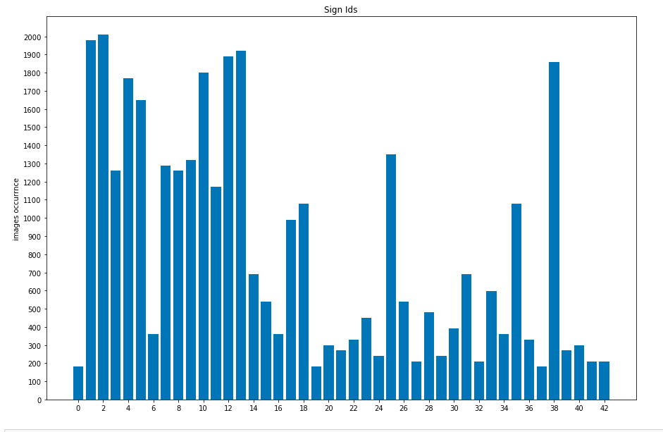
Here is an exploratory visualization of the data set. It is a bar chart showing how the data distribute
1. Describe how you preprocessed the image data. What techniques were chosen and why did you choose these techniques? Consider including images showing the output of each preprocessing technique. Pre-processing refers to techniques such as converting to grayscale, normalization, etc. (OPTIONAL: As described in the "Stand Out Suggestions" part of the rubric, if you generated additional data for training, describe why you decided to generate additional data, how you generated the data, and provide example images of the additional data. Then describe the characteristics of the augmented training set like number of images in the set, number of images for each class, etc.)
As a first step, I decided add additinal data because the variance between the dataset is very high which is 392816, and the mean is 809. Therefore, I decided to use agumtation in order to generate fake data. the imgaug library was chosen to facilitate the agumtation.
There were many techniques selected, look at augment_data(images) for more info. Here are some of them:
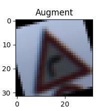
rotatation: to teach the network how to recover from a poor position.
CropAndPad: I put a small percetage (-0.25, 0.25) in order to make sure the sign still present on an image.
ChangeColorspace: I found that changing the color space it give a better result.
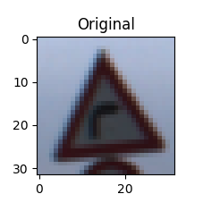
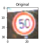
Here is an example of an original image and an augmented image:
The difference between the original data set and the augmented data set is the following
Number of old training examples is 34799
Number of new training examples is 125392 Image data shape is (125392, 32, 32, 3)
Old mean is 809
New mean is 2916
Old variance is 392816
New variance is 162136
| ClassID | Occurrences | Name |
|---|---|---|
| 25 | 3806 | Road work |
| 1 | 3683 | Speed limit (30km/h) |
| 13 | 3624 | Yield |
| 12 | 3551 | Priority road |
| 2 | 3478 | Speed limit (50km/h) |
| 9 | 3386 | No passing |
| 14 | 3298 | Stop |
| 38 | 3277 | Keep right |
| 7 | 3202 | Speed limit (100km/h) |
| 11 | 3196 | Right-of-way at the next intersection |
| 8 | 3164 | Speed limit (120km/h) |
| 31 | 3162 | Wild animals crossing |
| 4 | 3132 | Speed limit (70km/h) |
| 10 | 3123 | No passing for vehicles over 3.5 metric tons |
| 3 | 3054 | Speed limit (60km/h) |
| 33 | 3014 | Turn right ahead |
| 18 | 3010 | General caution |
| 15 | 2976 | No vehicles |
| 23 | 2970 | Slippery road |
| 16 | 2925 | Vehicles over 3.5 metric tons prohibited |
| 20 | 2885 | Dangerous curve to the right |
| 34 | 2835 | Turn left ahead |
| 24 | 2827 | Road narrows on the right |
| 29 | 2820 | Bicycles crossing |
| 22 | 2814 | Bumpy road |
| 5 | 2807 | Speed limit (80km/h) |
| 6 | 2760 | End of speed limit (80km/h) |
| 36 | 2750 | Go straight or right |
| 40 | 2748 | Roundabout mandatory |
| 35 | 2726 | Ahead only |
| 28 | 2725 | Children crossing |
| 17 | 2697 | No entry |
| 27 | 2693 | Pedestrians |
| 39 | 2668 | Keep left |
| 30 | 2665 | Beware of ice/snow |
| 26 | 2665 | Traffic signals |
| 21 | 2660 | Double curve |
| 19 | 2574 | Dangerous curve to the left |
| 41 | 2478 | End of no passing |
| 37 | 2238 | Go straight or left |
| 42 | 2170 | End of no passing by vehicles over 3.5 metric tons |
| 0 | 2168 | Speed limit (20km/h) |
| 32 | 1988 | End of all speed and passing limits |
As a second step, I normalized the image data by using (sklearn.preprocessing.scale function).
The reason behind normalization is that if a feature has a variance that is orders of magnitude larger than others, it may make the model unable to learn from other features correctly as expected.
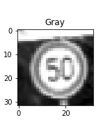
Lastly I decided to convert the image to grayscale because I want to teach the netwrok that colors do not matter on determining the trafic sign.
Here is an example of an original image and an gray image:
2. Describe what your final model architecture looks like including model type, layers, layer sizes, connectivity, etc.) Consider including a diagram and/or table describing the final model.
The model is same as LeNet-5 architecture except that I added dropout before the final fully connected layer.
My final model consisted of the following layers:
| Layer | Description |
|---|---|
| Input | 32x32x1 Gray image |
| Convolution 3x3 | 1x1 stride, VALID padding, outputs 28x28x6 |
| RELU | Activation function |
| Max pooling | 2x2 stride, outputs 14x14x6 |
| Convolution 3x3 | 1x1 stride, VALID padding, outputs 10x10x16 |
| RELU | Activation function |
| Max pooling | 2x2 stride, outputs 5x5x16 |
| Flatten | outputs 400 |
| Fully connected | outputs 120 |
| RELU | Activation function |
| Fully connected | outputs 80 |
| RELU | Activation function |
| dropout | 50% in order to smooth the traing |
| Fully connected | output = 43 |
3. Describe how you trained your model. The discussion can include the type of optimizer, the batch size, number of epochs and any hyperparameters such as learning rate.
Frist of all I used same parameters as the solution on LeNet-Lab. which has:
learning_rate = 0.001
epochs = 10
batch_size = 128
Then I played with these paramaters and my result is that
I select a random number for learning rate between (0.001, 0.0001). but it did not give much improvment on trained dataset.
For epochs, from 10 to 250 was selected, however, I found that for large data more than 70K it needs at least 25 to reach .93, since increasing the epochs it only result on overfitting most of the time.
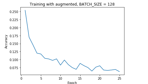
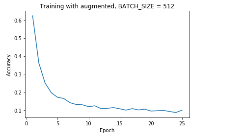
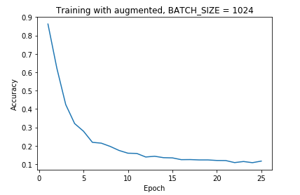
batch size 128 was good for the model to have a nice learning curave, because when I tried bigger batch size (256 - 1024), the model learn slower and did not give any improvement at all.
Here are some images to show different batch sizes were chosen
learning_rate = 0.001
epochs = 25
batch_size = 128
4. Describe the approach taken for finding a solution and getting the validation set accuracy to be at least 0.93. Include in the discussion the results on the training, validation and test sets and where in the code these were calculated. Your approach may have been an iterative process, in which case, outline the steps you took to get to the final solution and why you chose those steps. Perhaps your solution involved an already well known implementation or architecture. In this case, discuss why you think the architecture is suitable for the current problem.
My final model results were:
- training set accuracy of 0.986
- validation set accuracy of 0.9305
- test set accuracy of 0.906
If an iterative approach was chosen:
-
What was the first architecture that was tried and why was it chosen?
LeNet-5 was selected as it was recommended by Udacity and it was build for solving similar issues -
What were some problems with the initial architecture?
it gives the accuracy needed which was .93 after augment & apply pre-processing to data.
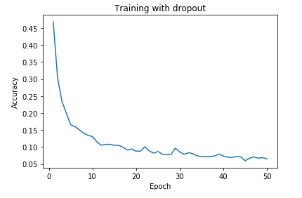
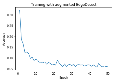
However, the initial architecture gaiv higher variance for accuracy.

Here are two examples: the seconde one is without using dropout
- How was the architecture adjusted and why was it adjusted? Typical adjustments could include choosing a different model architecture, adding or taking away layers (pooling, dropout, convolution, etc), using an activation function or changing the activation function. One common justification for adjusting an architecture would be due to overfitting or underfitting. A high accuracy on the training set but low accuracy on the validation set indicates over fitting; a low accuracy on both sets indicates under fitting.
I added dropout of .5 after the seconde fully connected layer
-
Which parameters were tuned? How were they adjusted and why?
None -
What are some of the important design choices and why were they chosen? For example, why might a convolution layer work well with this problem? How might a dropout layer help with creating a successful model?
convolution layer works best because it divided the features into smaller pieces.
And each convolution layer is responsible to identify some features.

For example, one convolution layer is responsible for identifing the left and right numbers in a trafic sign separately,
and another convolution layer would figure out the two number combination.
If a well known architecture was chosen:
- What architecture was chosen?
LeNet-5 - Why did you believe it would be relevant to the traffic sign application?
Since traffic sign application is basically a normal classification problem,
then LeNet-5 is a good initial architecture for starter to learn a simple architecture for solving a classification problem.
Also it gives the basic understanding of convolution neural network (CNN).
- How does the final model's accuracy on the training, validation and test set provide evidence that the model is working well?
Since the accuracy reach the requirements of this project then the model is working well
1. Choose five German traffic signs found on the web and provide them in the report. For each image, discuss what quality or qualities might be difficult to classify.
Here are five German traffic signs that I found on the web:
The pedestrians image might be difficult to classify because when I apply the augmentation to the dataset, the pedestrians trafic sign has many fake images from augmentation, it went from 210 to 2693 images.
2. Discuss the model's predictions on these new traffic signs and compare the results to predicting on the test set. At a minimum, discuss what the predictions were, the accuracy on these new predictions, and compare the accuracy to the accuracy on the test set (OPTIONAL: Discuss the results in more detail as described in the "Stand Out Suggestions" part of the rubric).
Here are the results of the prediction:
| Image | Prediction |
|---|---|
| Stop Sign | Stop sign |
| Speed limit (60km/h) | Speed limit (60km/h) |
| Road work | Road work |
| Pedestrians | Road narrows on the right |
| Keep right | Keep right |
The model was able to correctly guess 4 of the 5 traffic signs, which gives an accuracy of 80%. This compares favorably to the accuracy on the test set of 90%.
3. Describe how certain the model is when predicting on each of the five new images by looking at the softmax probabilities for each prediction. Provide the top 5 softmax probabilities for each image along with the sign type of each probability. (OPTIONAL: as described in the "Stand Out Suggestions" part of the rubric, visualizations can also be provided such as bar charts)
The code for making predictions on my final model is located in the 28th cell of the Ipython notebook.
For the first image, the model is relatively sure that this is a Speed limit (60km/h) sign (probability of 0.999), and the image does contain a Speed limit (60km/h) sign. The top five soft max probabilities were
| Probability | Prediction |
|---|---|
| 99.668% | Speed limit (60km/h) |
| 0.313% | Speed limit (80km/h) |
| 0.011% | Speed limit (50km/h) |
| 0.005% | No passing |
| 0.002% | Speed limit (30km/h) |
For the seconde image Road work
| Probability | Prediction |
|---|---|
| 99.999% | Road work |
| 0.001% | Bumpy road |
| 0.000% | Road narrows on the right |
| 0.000% | Bicycles crossing |
| 0.000% | Go straight or left |
For the third image Pedestrians
| Probability | Prediction |
|---|---|
| 99.667% | Road narrows on the right |
| 0.222% | Pedestrians |
| 0.069% | Bicycles crossing |
| 0.037% | Road work |
| 0.005% | Children crossing |
For the forth image Stop
| Probability | Prediction |
|---|---|
| 99.999% | Stop |
| 0.001% | Speed limit (120km/h) |
| 0.000% | Turn right ahead |
| 0.000% | Speed limit (60km/h) |
| 0.000% | No vehicles |
For the fifth image Keep right
| Probability | Prediction |
|---|---|
| 100.000% | Keep right |
| 0.000% | No entry |
| 0.000% | Bicycles crossing |
| 0.000% | Turn left ahead |
| 0.000% | Stop |
