Recursive functions are the natural way to express iterations in a functional programming langauge, but in R, they can be significantly slower than loop-versions and for moderately long sequences or moderately deep trees, recursive functions will reach a limit imposted on them by the stack limit.
There are known solutions to these problems, as long as functions are written to be tail-recursive, meaning that the return value of a function is either a base value or another recursive call, but where we do not call recursively to then do something with the result.
The goal of tailr is to automatically transform tail-recursive
functions into loops or trampolines.
You can install the released version of tailr from CRAN using
install.packages("tailr")You can install tailr from GitHub with:
# install.packages("devtools")
devtools::install_github("mailund/tailr")Consider a classical recursive function, factorial:
factorial <- function(n) {
    if (n <= 1) 1
    else n * factorial(n - 1)
}
(I know R already has a builtin factorial function, but please ignore
that). This function will compute the factorial of n, but if n is
too large, it will exceed the stack limit:
> factorial(3000)
Error: C stack usage  7970184 is too close to the limit
A classical way out of this problem is to turn it into a tail-recursive function:
factorial <- function(n, acc = 1) {
    if (n <= 1) acc
    else factorial(n - 1, acc * n)
}
R doesn’t implement the tail-recursion optimisation, though, so it doesn’t help us.
> factorial(3000)
Error: C stack usage  7970184 is too close to the limit
With tailr we can, automatically, translate a tail-recursive function
into a looping one, essentially implementing the tail-recursion
optimisation this way.
tr_factorial <- tailr::loop_transform(factorial, byte_compile = FALSE)I have disabled byte compilation to make running time comparisons fair
below; by default it is enabled. For a function as simple as
factorial, though, byte compiling will not affect the running time in
any substantial amount.
This version, because it looks instead of recurse, doesn’t have the stack limit problem:
tr_factorial(3000)
#> [1] Inf
We get the result Inf because the number we compute is too large to
represent on the computer, but that is not the point of the example. The
point is that the recursion doesn’t get too deep for the stack because
we avoid recursion alltogether.
With something as simple as computing the factorial, it is easy to write a looping function by hand, and it will be much faster than both the (tail-)recursive and the transformed function:
loop_factorial <- function(n) {
    val <- 1
    while (n > 1) {
        val <- n * val
        n <- n - 1
    }
    val
}


n <- 1000
bm <- microbenchmark::microbenchmark(factorial(n),
                                     tr_factorial(n),
                                     loop_factorial(n))
bm
#> Unit: microseconds
#>               expr     min        lq      mean   median       uq      max
#>       factorial(n) 753.327 1076.8550 1530.8461 1413.862 1933.627 7071.590
#>    tr_factorial(n) 891.502 1072.9835 1593.5777 1481.825 2105.525 4827.251
#>  loop_factorial(n)  60.654   64.7555  111.3827   74.984  113.365 2453.018
#>  neval
#>    100
#>    100
#>    100
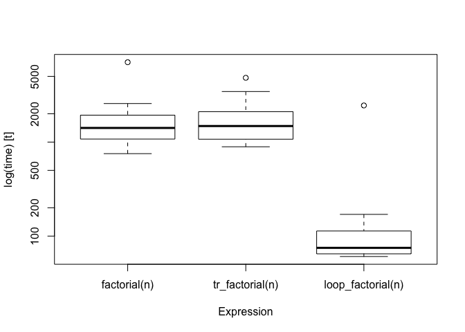
boxplot(bm)
The transformed version runs in about the same time as the recursive one, but the looping function is much faster.
However, consider a more complicated example. Using the pmatch
package, we can create a linked list data structure as this:
library(pmatch)
llist := NIL | CONS(car, cdr : llist)
A natural way to process linked lists using pattern matching is to write recursive functions that matches different patterns of their input. A function for computing the length of a linked list can look like this:
llength <- case_func(acc = 0,
   NIL -> acc,
   CONS(car, cdr) -> llength(cdr, acc + 1)
)
tr_llength <- tailr::loop_transform(llength)The function we generate is rather complicated
body(tr_llength)
#> .Primitive("{")(.tailr_.match_expr <- .match_expr, .tailr_acc <- acc,
#>     callCC(function(escape) {
#>         repeat {
#>             .Primitive("{")(.match_expr <- .tailr_.match_expr,
#>                 acc <- .tailr_acc, if (is.na(.match_expr) &&
#>                   attr(.match_expr, "constructor") == "NIL")
#>                   escape(acc)
#>                 else if ({
#>                   .cons <- attr(.match_expr, "constructor")
#>                   !is.null(.cons) && .cons == "CONS"
#>                 } && {
#>                   car <- .match_expr$car
#>                   TRUE
#>                 } && {
#>                   cdr <- .match_expr$cdr
#>                   TRUE
#>                 }) {
#>                   .tailr_.match_expr <<- cdr
#>                   .tailr_acc <<- acc + 1
#>                 }
#>                 else {
#>                   escape(stop("None of the patterns match."))
#>                 }, next)
#>         }
#>     }))
but, then, it is not one we want to manually inspect in any case.
It is not too hard to implement this function with a loop either, but it is not as simple as the recursive function:
is_nil <- case_func(NIL -> TRUE, otherwise -> FALSE)
loop_llength <- function(llist) {
    len <- 0
    while (!is_nil(llist)) {
        len <- len + 1
        llist <- llist$cdr
    }
    len
}
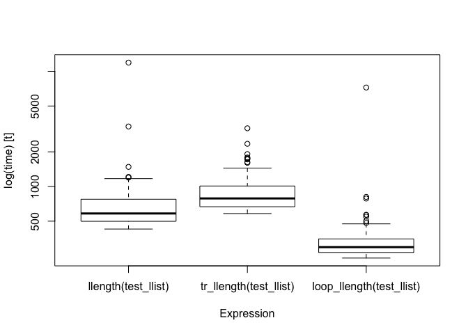
If we compare the running time for these three functions, the transformed function is faster than the recursive but not as fast as the iterative:
make_llist <- function(n) {
    l <- NIL
    for (i in 1:n) {
        l <- CONS(i, l)
    }
    l
}
test_llist <- make_llist(100)
bm <- microbenchmark::microbenchmark(llength(test_llist),
                                     tr_llength(test_llist),
                                     loop_llength(test_llist))
bm
#> Unit: microseconds
#>                      expr     min       lq     mean   median        uq
#>       llength(test_llist) 427.303 498.6945 792.0072 583.1925  775.2950
#>    tr_llength(test_llist) 582.458 667.3435 924.0303 787.9700 1010.1635
#>  loop_llength(test_llist) 239.194 267.5165 398.4339 297.4250  350.5305
#>        max neval
#>  11909.065   100
#>   3202.308   100
#>   7234.805   100
boxplot(bm)
FIXME: The main reason for this is that the running time is
dominated by the cost of pmatch. If I manage to get that faster, the
iterative function might end being much faster here as well.
More examples:
llcontains <- case_func(x,
    NIL -> FALSE,
    CONS(car, cdr) -> if (car == x) TRUE else llcontains(cdr, x)
)

tr_llcontains <- tailr::loop_transform(llcontains)

loop_contains <- function(lst, x) {
    while (!is_nil(lst)) {
        if (x == lst$car) return(TRUE)
        else lst <- lst$cdr
    }
}

lst <- make_llist(100)
bm <- microbenchmark::microbenchmark(llcontains(lst, 1001),
                                     tr_llcontains(lst, 1001),
                                     loop_contains(lst, 1001))
bm
#> Unit: microseconds
#>                      expr     min       lq     mean  median       uq
#>     llcontains(lst, 1001) 416.362 463.1385 595.6020 491.507 528.2700
#>  tr_llcontains(lst, 1001) 602.532 664.2220 763.1534 692.794 746.6635
#>  loop_contains(lst, 1001) 337.272 357.2140 463.2347 381.119 413.5190
#>       max neval
#>  8220.268   100
#>  3590.782   100
#>  4011.447   100
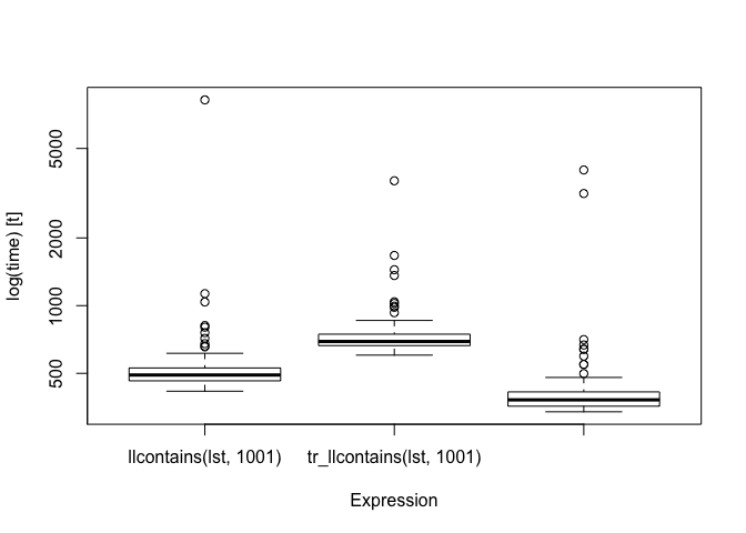
boxplot(bm)
llrev <- pmatch::case_func(acc = NIL,
NIL -> acc,
CONS(car, cdr) -> llrev(cdr, CONS(car, acc))
)
bubble <- case_func(swapped = FALSE, acc = NIL,
CONS(first, CONS(second, rest)) ->
if (first > second) bubble(CONS(first, rest), TRUE, CONS(second, acc))
else bubble(CONS(second, rest), swapped, CONS(first, acc)),
CONS(x, NIL) -> list(new_list = llrev(CONS(x, acc)), swapped = swapped)
)
bubble_sort <- function(lst) {
if (is_nil(lst)) return(lst)
bind[lst, swapped] <- bubble(lst)
while (swapped) {
bind[lst, swapped] <- bubble(lst)
}
lst
}
lst <- CONS(3, CONS(2, CONS(5, CONS(1, NIL))))
bubble_sort(lst)
#> CONS(car = 1, cdr = CONS(car = 2, cdr = CONS(car = 3, cdr = CONS(car = 5, cdr = NIL))))tr_llrev <- pmatch::case_func(acc = NIL,
NIL -> acc,
CONS(car, cdr) -> llrev(cdr, CONS(car, acc))
)
tr_llrev <- tailr::loop_transform(tr_llrev)
tr_bubble <- case_func(swapped = FALSE, acc = NIL,
CONS(first, CONS(second, rest)) ->
if (first > second) tr_bubble(CONS(first, rest), TRUE, CONS(second, acc))
else tr_bubble(CONS(second, rest), swapped, CONS(first, acc)),
CONS(x, NIL) -> list(new_list = tr_llrev(CONS(x, acc)), swapped = swapped)
)
tr_bubble <- tailr::loop_transform(tr_bubble)
tr_bubble_sort <- function(lst) {
if (is_nil(lst)) return(lst)
bind[lst, swapped] <- tr_bubble(lst)
while (swapped) {
bind[lst, swapped] <- tr_bubble(lst)
}
lst
}
lst <- CONS(3, CONS(2, CONS(5, CONS(1, NIL))))
tr_bubble_sort(lst)
#> CONS(car = 1, cdr = CONS(car = 2, cdr = CONS(car = 3, cdr = CONS(car = 5, cdr = NIL))))loop_llrev <- function(lst) {
acc <- NIL
while (!is_nil(lst)) {
acc <- CONS(lst$car, acc)
lst <- lst$cdr
}
acc
}
loop_bubble <- function(lst, swapped = FALSE) {
acc <- NIL
repeat {
if (is_nil(lst$cdr))
return(list(new_list = loop_llrev(CONS(lst$car, acc)),
swapped = swapped))
first <- lst$car
second <- lst$cdr$car
rest <- lst$cdr$cdr
if (first > second) {
acc <- CONS(second, acc)
lst <- CONS(first, rest)
swapped <- TRUE
} else {
acc <- CONS(first, acc)
lst <- CONS(second, rest)
}
}
}
loop_bubble_sort <- function(lst) {
if (is_nil(lst)) return(lst)
bind[lst, swapped] <- loop_bubble(lst)
while (swapped) {
bind[lst, swapped] <- loop_bubble(lst)
}
lst
}
lst <- CONS(3, CONS(2, CONS(5, CONS(1, NIL))))
loop_bubble_sort(lst)
#> CONS(car = 1, cdr = CONS(car = 2, cdr = CONS(car = 3, cdr = CONS(car = 5, cdr = NIL))))lst <- make_llist(10)
bm <- microbenchmark::microbenchmark(bubble_sort(lst),
tr_bubble_sort(lst),
loop_bubble(lst))
bm
#> Unit: microseconds
#> expr min lq mean median uq
#> bubble_sort(lst) 4041.428 4362.236 5023.292 4688.6965 5461.7020
#> tr_bubble_sort(lst) 4545.728 4799.363 5563.993 5084.3145 5753.0465
#> loop_bubble(lst) 132.440 150.315 179.494 160.7555 173.8895
#> max neval
#> 8529.733 100
#> 11671.375 100
#> 536.358 100
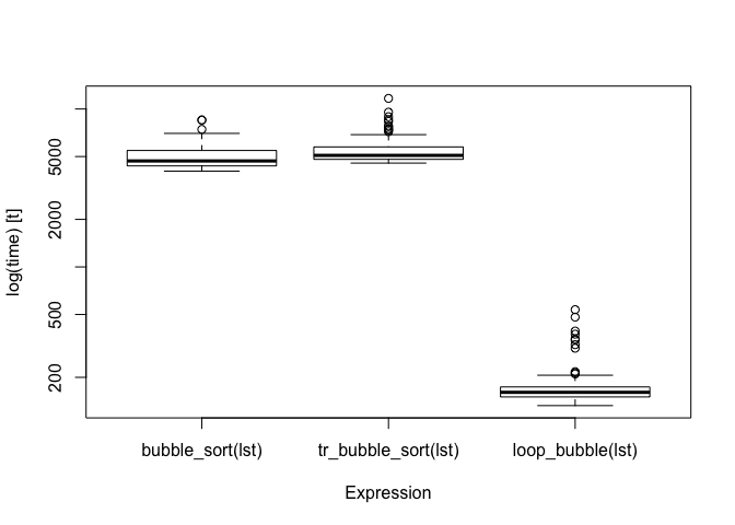
boxplot(bm)The module primarily solves the problem of exceeding the stack space. The transformed functions are not as fast as those we can code by hand using loops. It should be possible to improve on the running time of the transformed functions, however, with some program analysis… This analysis should be included in the time usage analysis, though, which will probably still come out saying that manually programmed looping versions are faster than transformed functions. Recursive functions can be a lot easier to read, though, than their corresponding looping versions, especially with pattern matching.


