magnusdv / pedbuildr

Pedigree Reconstruction in R

pedbuildr

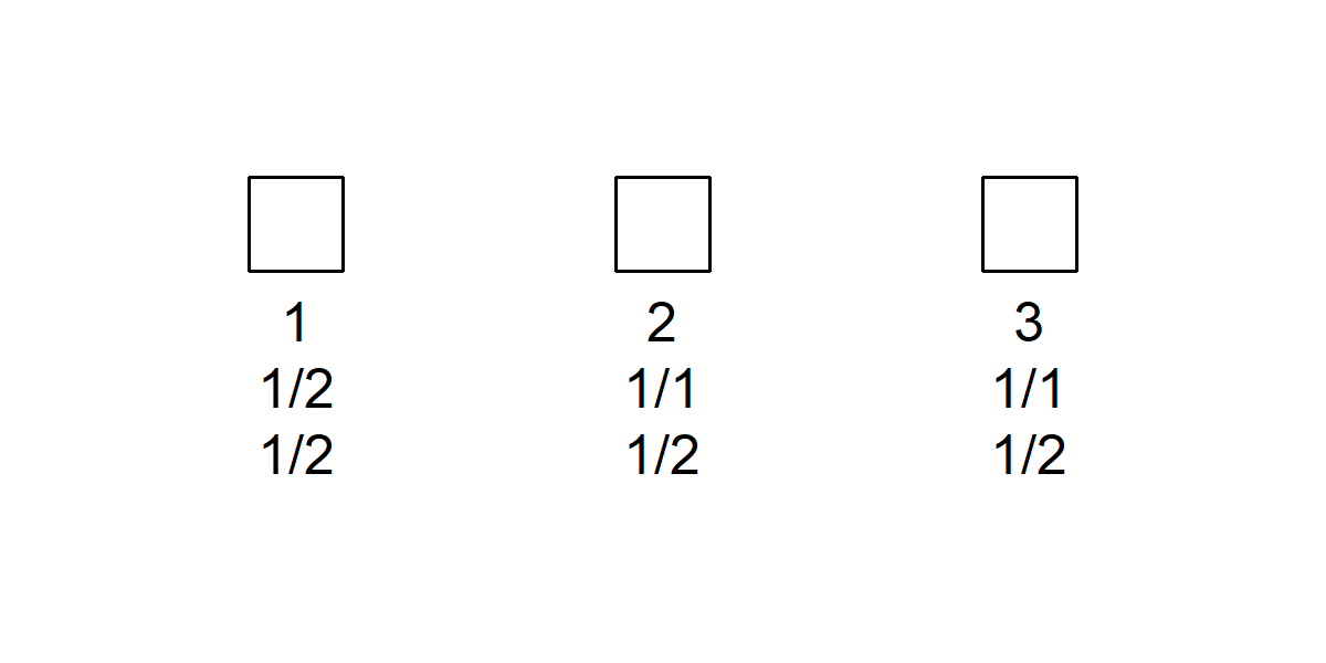
The goal of pedbuildr is to reconstruct pedigrees from genotype data. This is done by optimising the likelihood over all possible pedigrees subject to given restrictions. As part of the pedsuite ecosystem of R packages for pedigree analysis, it uses pedtools for handling pedigrees, and imports pedprobr for calculating pedigree likelihoods.

See also the ibdEstimate() function of forrel, which does pairwise relatedness estimation.

Installation

The pedbuildr package can be installed from CRAN as follows:

install.packages("pedbuildr")

Alternatively, the latest development version is available from GitHub.

# install.packages("devtools")
devtools::install_github("magnusdv/pedbuildr")

A reconstruction example

To get started, load pedbuildr.

library(pedbuildr)
#> Loading required package: pedtools

The built-in dataset trioData contains simulated genotypes for three individuals at 100 equifrequent SNP markers. Here are the first 10 columns:

trioData[, 1:10]
#>   <1>   <2>   <3>   <4>   <5>   <6>   <7>   <8>   <9>   <10> 
#> 1 "1/2" "1/2" "1/1" "1/2" "1/2" "1/2" "1/2" "2/2" "1/2" "1/2"
#> 2 "1/1" "1/2" "1/2" "2/2" "1/2" "2/2" "1/2" "2/2" "1/2" "2/2"
#> 3 "1/1" "1/2" "1/2" "2/2" "1/1" "1/2" "1/2" "1/2" "1/2" "2/2"

As a simple demonstration we will try to reconstruct the pedigree connecting these individuals assuming they are all males. To initialise the process we create them as singletons and attach the marker data. The locusAttributes argument tells R that all the markers are diallelic with alleles 1 and 2.

x = list(singleton(1), 
         singleton(2), 
         singleton(3)) |> 
  setMarkers(alleleMatrix = trioData, locusAttributes = "snp12")

plotPedList(x, frames = FALSE)

To reconstruct the pedigree, simply run reconstruct():

res = reconstruct(x)
#> Pedigree parameters:
#>   ID labels: 1, 2, 3
#>   Sex: 1, 1, 1
#>   Extra: parents
#>   Age info: -
#>   Known PO: -
#>   Known non-PO: -
#>   No children: -
#>   Connected only: TRUE
#>   Symmetry filter: TRUE
#>   Max inbreeding: 0.0625
#>   Linear inbreeding: FALSE
#> 
#> Building pedigree list:
#>   Undirected adjacency matrices: 8 
#>   Directed adjacency matrices: 16 
#>   After adding parents: 57 
#>   Connected solutions: 44 
#>   Excessive inbreeding: 0 
#> 
#> Computing the likelihood of 44 pedigrees.
#> Sorting by descending likelihood.
#> Total time used:  1.6 secs

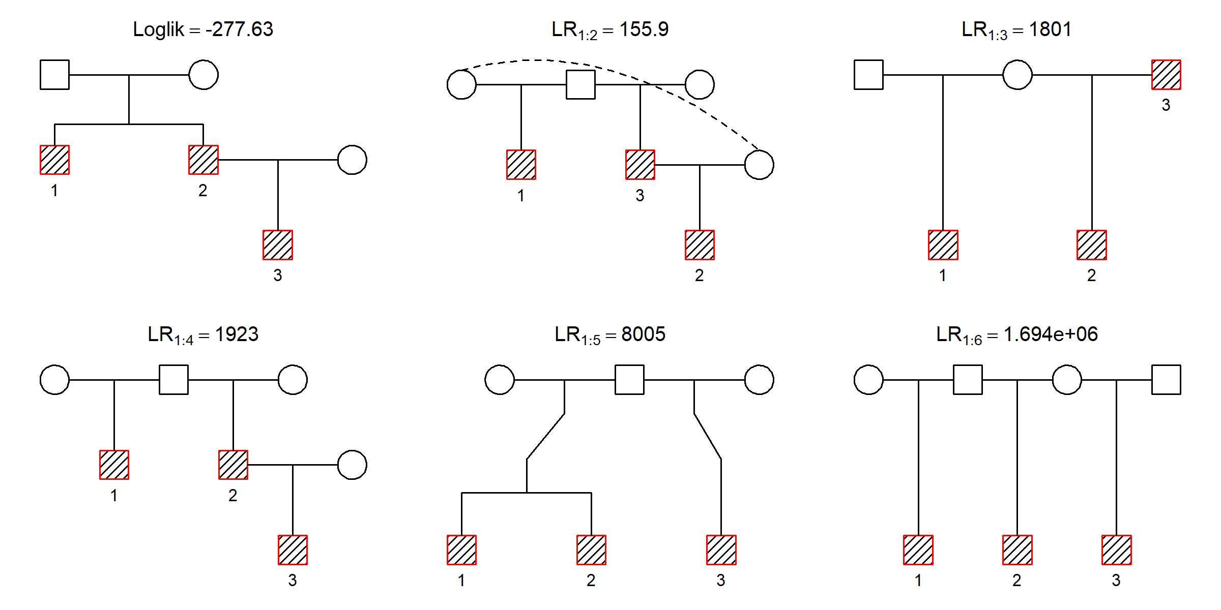
A tailor-made plot function makes it easy to visualise the most likely pedigrees:

plot(res, top = 6)

The most likely pedigree is plotted top left. The titles for the remaining pedigrees give the likelihood ratio (LR) comparing the first pedigree to the one shown. For example, the first solution is 155.9 more likely than the second.

Further options

A priori there are infinitely many possible pedigrees connecting a set of individuals. (For example, two individuals may be k’th cousins for any k = 1,2,… .) In order to obtain a manageable search space, reconstruct() offers a range of restriction parameters:

• extra: The number of extra individuals allowed to connect the original individuals. (See further explanations below.)
• age: A vector of numeric (relative) ages or age inequalities. For example, age = c("A > B,C", "B > D") excludes B and C as ancestors of A, and D as an ancestor of B (but no assumption is made for C vs. D).
• inferPO: When this is TRUE, an initial pairwise estimation step is done to infer high-confidence parent/child pairs, and also non-parent/child pairs.
• knownPO: Known parent–offspring pairs. Note that these are unordered pairs, i.e., with no assumption on who is the parent and who is the child. (If this is known, use age to indicate it.)
• notPO: Pairs known not to be parent–offspring.
• allKnown: If TRUE, then knownPO is taken to be the complete list of parent–offspring pairs.
• noChildren: Individuals known to have no children.
• maxInbreeding: The highest permitted inbreeding coefficient in the pedigree. By default this is set to 1/16, which is appropriate for most projects involving human pedigrees.
• linearInb: The allowed level of inbreeding between linear descendants. For example, linearInb = 1 allows mating between parent–child, but not grandparent–grandchild. The default value FALSE disallows all inbreeding of this type.
• connected: If TRUE (default), only connected pedigrees are considered.
• sexSymmetry: If TRUE (default) pedigrees are considered equal if they differ only in the sexes of the added parents, e.g., paternal versus maternal half-siblings.

Let us re-run the reconstruction of trioData adding a few of these restrictions. We allow 3 extra individuals and indicate that individual 1 is older than the others. Furthermore, we ask the program to infer parent-child relationships automatically. Finally we allow any amount of inbreeding.

res2 = reconstruct(x, extra = 3, age = "1 > 2,3", inferPO = TRUE, maxInbreeding = 1)
#> Pairwise estimation:
#>   PO: 2-3 
#>   non-PO: 1-3 
#> 
#> Pedigree parameters:
#>   ID labels: 1, 2, 3
#>   Sex: 1, 1, 1
#>   Extra: 3
#>   Age info: 1>2, 1>3
#>   Known PO: 2-3
#>   Known non-PO: 1-3
#>   No children: -
#>   Connected only: TRUE
#>   Symmetry filter: TRUE
#>   Max inbreeding: 1
#>   Linear inbreeding: FALSE
#> 
#> Building pedigree list:
#>   First 2: 2 candidates (0.0027 secs)
#>   All 3 + 0 extra: 1 solutions | 3 candidates (0.00353 secs)
#>   All 3 + 1 extra: 9 solutions | 30 candidates | 21 duplicates removed (0.0491 secs)
#>   All 3 + 2 extra: 35 solutions | 266 candidates | 501 duplicates removed (0.221 secs)
#>   All 3 + 3 extra: 183 solutions | 183 candidates | 459 duplicates removed (0.842 secs)
#>   Total solutions: 228 
#>   Converting to ped
#>   Excessive inbreeding: 0 
#>   Time used: 1.07 secs 
#> 
#> Computing the likelihood of 228 pedigrees.
#> Sorting by descending likelihood.
#> Total time used:  18.1 secs

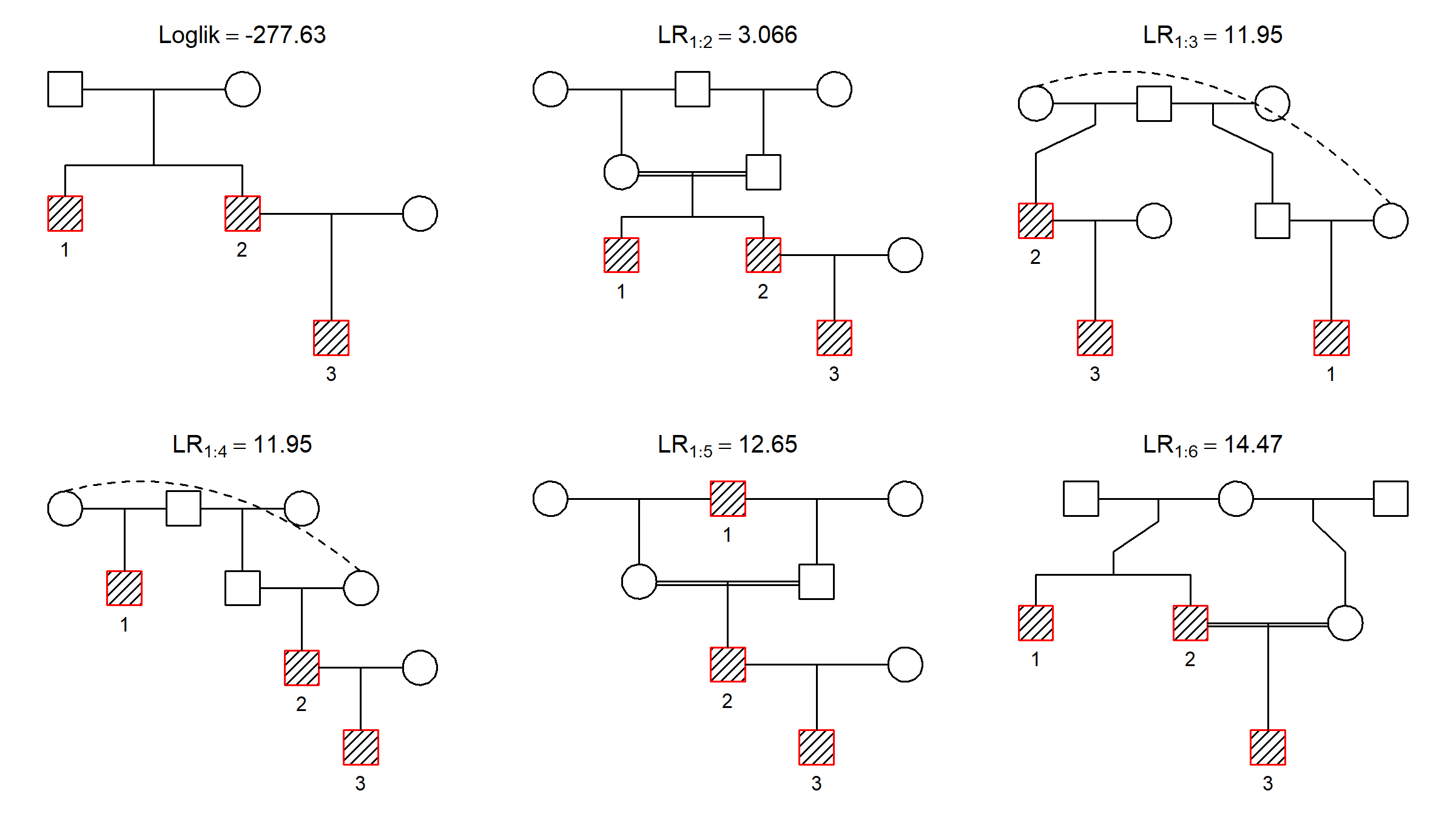
The most likely results this time are shown below:

plot(res2, top = 6)

We see that the same pedigree “wins”, but some inbred/esoteric alternatives have appeared among the runners-up.

More about extra

Arguably the most important parameter to reconstruct() is extra, which controls the size of the pedigrees to consider. It can be either a nonnegative integer, or the word “parents”. If an integer, it sets the maximum number of extra members used to connect the original individuals. (The final pedigrees may contain further extras still, since missing parents are added at the end.)

If extra = "parents", a special algorithm is invoked. First all directed acyclic graphs between the original individuals are generated, and then parents are added in all possible ways. This is (currently) the default behaviour, since it avoids setting an ad hoc number of “extras”. However, it only works well in relatively small cases.