machkev / LSTM_stock_price_predictor

Create deep learning models using LSTM RNN to predict cryptocurrency price.

Build and Evaluate Deep Learning Models

Overview

In this project we will develop and evaluate two custom Long Short-Term Memory Recurrent Neural Network models that predict Bitcoin nth day closing price based on a rolling X day window. The first model will use the Crypto Fear and Greed Index (FNG), which analyzes emotions and sentiments from different sources to produce a daily FNG value for cryptocurrencies. The second model will use Bitcoin closing prices. During training we will experiment with different values for the following parameters: window size(lookback window), number of input layers, number of epochs, and batch size. Each model will be evaluated on test data(unseen data). This process can be repeated multiple times until we find a model with the best performace. Then use the model to make predictions and compare them to actual values.

Note: Each model will be built in separate notebooks. In order to make accurate comparisons between the two models, we need to maintain the same architecture and parameters during training and testing of each model.

Preprocessing the data for training and testing

After importing and munging the data, each model will use 70% for training and 30% for testing.

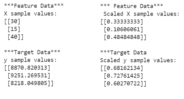
In order to deal with possible outlier values and avoid skewed models, we need to apply the MinMaxScaler function from sklearn.preprocessing tools to scale both x and y. This will arrange the feature and target values between 0 and 1, which will lead to more accurate predictions.

Note: It is good practice to fit the preprocessing function with the training dataset only. This will prevent look-ahead bias.

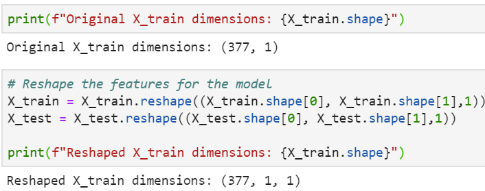
The LSTM model requires the input to every layer to be in a 3D matrix format. These three dimensions are (samples, time steps, features). We can convert the data by using the numpy.reshape function.

Build and train the LSTM RNN

To begin designing a custom LSTM RNN we need to import the following modules:

from tensorflow.keras.models import Sequential 
from tensorflow.keras.layers import Dense, LSTM, Dropout

The Sequential model allows us to add and/or decrease stacks of LSTM layers. Each layer is able to identify and extract different patterns of time series sequences. The Dropout layer is a regularization method that reduces overfitting and improves performance by randomly dropping a fraction of the nodes created by the LSTM layer. The Dense layer "specifies the dimensionality of the output space". In this project the last layer flattens out the results from all the layers above and gives a single prediction.

After designing the model, we are ready to compile and fit it with our training dataset. It is here where we can further optimize our model by experimenting with the fit function parameters. We can refer to the official Keras guide for an in-depth explanation of the LSTM RNN.

The snapshot below summarizes the architecture that resulted in the best performance for both the FNG and closing price models.

window_size = 1 
number_units = 30 # LSTM cells that learn to remember which historical patterns are important. 
drop_out_franction = 0.2 # 20% of neurons will be randomly dropped during each epoch
model = Sequential()
# add 1st layer
model.add(LSTM(units = number_units, 
              return_sequences = True,  
              input_shape = (X_train.shape[1],1)
         ))
model.add(Dropout(drop_out_franction))
# add 2nd layer
model.add(LSTM(units = number_units, return_sequences=True))
model.add(Dropout(drop_out_franction))
# add 3rd layer 
model.add(LSTM(units = number_units))
model.add(Dropout(drop_out_franction))
# add output layer
model.add(Dense(units=1))
# Compile the model
model.compile(loss='mean_squared_error', optimizer='adam', metrics=['mse'])
model.fit(X_train,y_train, epochs =50, batch_size=10, verbose = 0, shuffle=False)

Evaluating the performance of each model

In this section we will use X_test data to evaluate the performance and make predictions for each model. Then we will create a Dataframe to compare real prices vs predicted prices. One important step here is to use the scaler.inverse transform function to recover the actual closing prices from the scaled values.

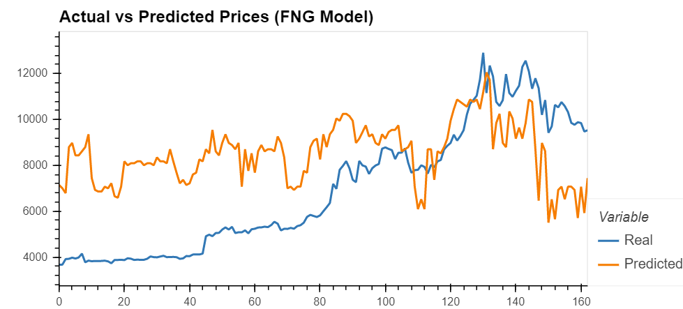
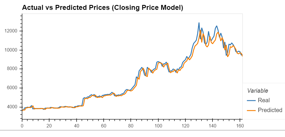
Once the building, training, and testing proceedures have been successfully completed, we can see that the closing price model resulted in more accurate predictions. This is supported by the mean square error loss metric. The FNG model has a loss of .1283, and the closing price model has a lower loss of .0025. We can better visualize the performance by using a line chart to compare the real with the actual closing prices.