The movie of 80 ribosome along PC1
mov4.mp4
This repository contains the implementation of opus-deep structural disentanglement (DSD), which is developed by the research group of Prof. Jianpeng Ma at Fudan University. The publication of this method is available at https://www.nature.com/articles/s41592-023-02031-6. A newer version with better reconstruction quality is available upon request. An exemplar movie of the new version is shown below:
mov1.mp4
This program is built upon a set of great works:
This project seeks to unravel how a latent space, encoding 3D structural information, can be learned utilizing only 2D image supervisions which are aligned against a consensus reference model.
An informative latent space is pivotal as it simplifies data analysis by providing a structured and reduced-dimensional representation of the data.
Our approach strategically leverages the inevitable pose assignment errors introduced during consensus refinement, while concurrently mitigating their impact on the quality of 3D reconstructions. Although it might seem paradoxical to exploit errors while minimizing their effects, our method has proven effective in achieving this delicate balance.
The workflow of this method is demonstrated as follows:
Note that all input and output of this method are in real space! (Fourier space is good, but how about real space!) The architecture of encoder is (Encoder class in cryodrgn/models.py):
The architecture of decoder is (ConvTemplate class in cryodrgn/models.py. In this version, the default size of output volume is set to 192^3, I downsampled the intermediate activations to save some gpu memories. You can tune it as you wish, happy training!):
The weight file can be downloaded from https://www.icloud.com/iclouddrive/0fab8AGmWkNjCsxVpasi-XsGg#weights.
The other pkls for visualzing are deposited at https://drive.google.com/drive/folders/1D0kIP3kDhlhRx12jVUsZUObfHxsUn6NX?usp=share_link.
These files are from the epoch 16 and trained with output volume of size 192. z.16.pkl stores the latent encodings for all particles. ribo_pose_euler.pkl is the pose parameter file. Our program will read configurations from config.pkl. Put them in the same folder, you can then follow the analyze result section to visualize the latent space.
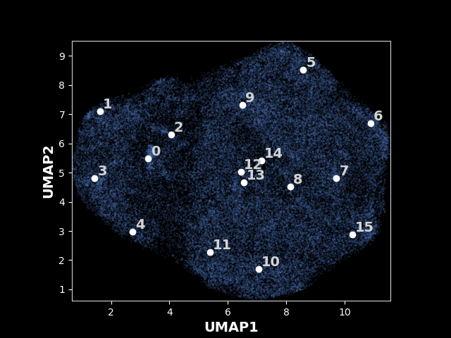
An exmaple UMAP of latent space for 80S ribosome:
Comparison between some states:

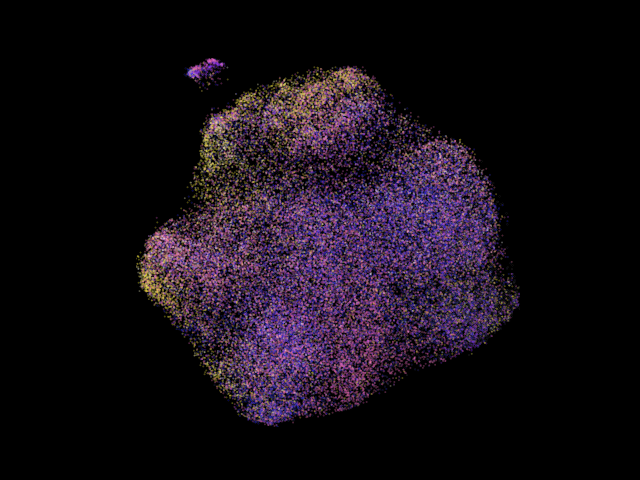
A more colorful one, the particles are colored according to their projection classes, note the clusters often show certain dominant colors, this is due to the consensus refinement will account structural variations in images by distorting their pose paramters like fitting a longer rod into a small gap by tilting the rod! (those are all what the consensus refinement can fit!)
Data source: EMPIAR-10002. The particles are colored according to their pose parameters in this image.
UMAP and some selected classes for the spliceosome complex

The movie of the movement in spliceosome along PC1
mov1.mp4
After cloning the repository, to run this program, you need to have an environment with pytorch and a machine with GPUs. The recommended configuration is a machine with 4 V100 GPUs. You can create the conda environment for DSD using the spec-file in the folder and by executing
conda create --name dsd --file spec-file
or using the environment.yml file in the folder by executing
conda env create --name dsd -f environment.yml
After the environment is sucessfully created, you can then activate it and execute our program within this environement.
conda activate dsd
The inference pipeline of our program can run on any GPU which supports cuda 10.2 and is fast to generate a 3D volume. However, the training of our program takes larger amount memory, we recommend using V100 GPUs at least.
This program is developed based on cryoDRGN and adheres to a similar data preparation process.
Data Preparation Guidelines:
-
Cryo-EM Dataset: Ensure that the cryo-EM dataset is stored in the MRCS stack file format. A good dataset for tutorial is the splicesome which is available at https://empiar.pdbj.org/entry/10180/ (It contains the consensus refinement result.)
-
Consensus Refinement Result: The program requires a consensus refinement result, which should not apply any symmetry and must be stored as a Relion STAR file. Other 3D reconstruction results such as 3D classification, as long as they determine the pose parameters of images, can also be supplied as input.
Usage Example:
Assuming the refinement result is stored as run_data.star and the format of the Relion STAR file is below version 3.0,
You can then prepare the pose parameter file by executing the below command inside the opus-dsd folder:
python -m cryodrgn.commands.parse_pose_star /work/run_data.star -D 192 --Apix 1.35 -o hrd-pose-euler.pkl
suppose the run_data.star is located at /work/ directory, where
| argument | explanation |
|---|---|
| -D | the dimension of the particle image in your dataset |
| --Apix | is the angstrom per pixel of you dataset |
| -o | followed by the filename of pose parameter used by our program |
| --relion31 | include this argument if you are using star file from relion with version higher than 3.0 |
Next, you can prepare the ctf parameter file by executing:
python -m cryodrgn.commands.parse_ctf_star /work/run_data.star -D 192 --Apix 1.35 -o hrd-ctf.pkl -o-g hrd-grp.pkl --ps 0
| argument | explanation |
|---|---|
| -o-g | used to specify the filename of ctf groups of your dataset |
| --ps | used to specify the amount of phaseshift in the dataset |
For star file from relion with version hgiher than 3.0, you should add --relion31 and more arguments to the command line!
Checkout prepare.sh which combine both commands to save your typing.
Finally, you should create a mask using the consensus model and RELION as in the postprocess. Suppose the filename of mask is mask.mrc, move it to the program directory for simplicity.
After executing all these steps, you have three pkls for running opus-DSD in the program directory ( You can specify any directories you like in the command arguments ).
When the pkls are available, you can then train the vae for structural disentanglement proposed in DSD using
python -m cryodrgn.commands.train_cv /work/hrd.mrcs --ctf ./hrd-ctf.pkl --poses ./hrd-pose-euler.pkl --lazy-single --pe-type vanilla --encode-mode grad --template-type conv -n 20 -b 18 --zdim 8 --lr 1.e-4 --num-gpus 4 --multigpu --beta-control 1. --beta cos -o /work/hrd -r ./mask.mrc --downfrac 0.9 --lamb 1. --split hrd-split.pkl --bfactor 4. --templateres 192
The second argument after train_cv specified the path of image stack.
The three arguments --pe-type vanilla --encode-mode grad --template-type conv ensure OPUS-DSD is enabled! The default values are setting to them in our program, you can ommit them incase of simplicity.
The function of each argument is explained as follows:
| argument | explanation |
|---|---|
| --ctf | ctf parameters of the image stack |
| --poses | pose parameters of the image stack |
| -n | the number of training epoches, each training epoch loops through all images in the training set |
| -b | the number of images for each batch on each gpu, depends on the size of available gpu memory |
| --zdim | the dimension of latent encodings, increase the zdim will improve the fitting capacity of neural network, but may risk of overfitting |
| --lr | the initial learning rate for adam optimizer, 1.e-4 should work, but you may use larger lr for dataset with higher SNR |
| --num-gpus | the number of gpus used for training, note that the total number of images in the total batch will be n*num-gpus |
| --multigpu | toggle on the data parallel version |
| --beta-control | the restraint strength of the beta-vae prior, the larger the argument, the stronger the restraint. The scale of beta-control should be propotional to the SNR of dataset. Suitable beta-control might help disentanglement by increasing the magnitude of latent encodings and the sparsity of latent encodings, for more details, check out beta vae paper. In our implementation, we adjust the scale of beta-control automatically based on SNR estimation, possible ranges of this argument are [0.5-4.]. You can use larger beta-control for dataset with higher SNR |
| --beta | the schedule for restraint stengths, cos implements the cyclic annealing schedule and is the default option |
| -o | the directory name for storing results, such as model weights, latent encodings |
| -r | the solvent mask created from consensus model, our program will focus on fitting the contents inside the mask (more specifically, the 2D projection of a 3D mask). Since the majority part of image dosen't contain electron density, using the original image size is wasteful, by specifying a mask, our program will automatically determine a suitable crop rate to keep only the region with densities. |
| --downfrac | the downsampling fraction of image, the reconstruction loss will be computed using the downsampled image of size D*downfrac. You can set it according to resolution of consensus model. We only support D*downfrac >= 128 so far (I may fix this behavior later) |
| --lamb | the restraint strength of structural disentanglement prior proposed in DSD, set it according to the SNR of your dataset, for dataset with high SNR such as ribosome, splicesome, you can safely set it to 1., for dataset with lower SNR, consider lowering it. Possible ranges are [0.2, 2.] |
| --split | the filename for storing the train-validation split of image stack |
| --valfrac | the fraction of images in the validation set, default is 0.1 |
| --bfactor | will apply exp(-bfactor/4 * s^2 * 4*pi^2) decaying to the FT of reconstruction, s is the magnitude of frequency, increase it leads to sharper reconstruction, but takes longer to reveal the part of model with weak density since it actually dampens learning rate, possible ranges are [3, 8]. Consider using higher values for more dynamic structures. We will decay the bfactor every epoch. This is equivalent to learning rate warming up. |
| --templateres | the size of output volume of our convolutional network, it will be further resampled by spatial transformer before projecting to 2D images. The default value is 192. You can tweak it to other resolutions, larger resolutions can generate sharper density maps |
| --plot | you can also specify this argument if you want to monitor how the reconstruction progress, our program will display the 2D reconstructions and experimental images after 8 times logging intervals |
| --tmp-prefix | the prefix of intermediate reconstructions, default is tmp |
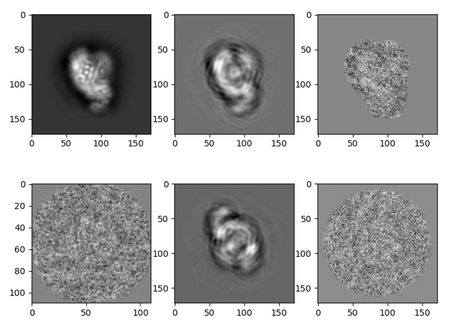
The plot mode will display the following images:
 Each row shows a selected image and its reconstruction from a batch.
In the first row, the first image is a 2D projection, the second image is a 2D reconstruction blurred by the corresponding CTF, the third image is the correpsonding experimental image after 2D masking.
In the second row, the first image is the experimental image supplemented to encoder, the second image is the 2D reconstruction, the third image is the correpsonding experimental image without masking.
You can use nohup to let the above command execute in background and use redirections like 1>log 2>err to redirect ouput and error messages to the corresponding files.
Happy Training! Contact us when running into any troubles.
To restart execution from a checkpoint, you can use
python -m cryodrgn.commands.train_cv hrd.txt --ctf ./hrd-ctf.pkl --poses ./hrd-pose-euler.pkl --lazy-single -n 20 --pe-type vanilla --encode-mode grad --template-type conv -b 18 --zdim 8 --lr 1.e-4 --num-gpus 4 --multigpu --beta-control 1. --beta cos -o /work/output -r ./mask.mrc --downfrac 0.9 --lamb 1. --load /work/hrd/weights.0.pkl --latents /work/hrd/z.0.pkl --split hrd-split.pkl --bfactor 6.
| argument | explanation |
|---|---|
| --load | the weight checkpoint from the restarting epoch |
| --latents | the latent encodings from the restarting epoch |
boths are in the output directory
During training, opus-DSD will output temporary volumes called tmp*.mrc (or the prefix you specified), you can check out the intermediate results by viewing them in Chimera. Opus-DSD uses 3D volume as intermediate representation, so it requires larger amount of memory, v100 gpus will be sufficient for its training. Its training speed is slower, which requires 2 hours on 4 v100 gpus to finish one epoch on dataset with 20k images. Opus-DSD also reads all images into memory before training, so it may require some more host memories (but this behavior can be toggled off, i didn't add an argument yet)
You can use the analysis scripts in opusDSD to visualizing the learned latent space! The analysis procedure is detailed as following.
The first step is to sample the latent space using kmeans algorithm. Suppose the results are in ./data/ribo,
sh analyze.sh ./data/ribo 16 2 16
- The first argument after
analyze.shis the output directory used in training, which storesweights.*.pkl, z.*.pkl, config.pkl - the second argument is the epoch number you would like to analyze,
- the third argument is the number of PCs you would like to sample for traversal
- the final argument is the number of clusters for kmeans clustering.
The analysis result will be stored in ./data/ribo/analyze.16, i.e., the output directory plus the epoch number you analyzed, using the above command. You can find the UMAP with the labeled kmeans centers in ./data/ribo/analyze.16/kmeans16/umap.png and the umap with particles colored by their projection parameter in ./data/ribo/analyze.16/umap.png .
After running the above command once, you can skip umap embedding step by appending the command in analyze.sh with --skip-umap. Our analysis script will read the pickled umap embeddings directly.
You can generate the volume which corresponds to each cluster centroid or traverses the principal component using, (you can check the content of scirpt first, there are two commands, one is used to evaluate volume at kmeans center, another one is for PC traversal, just choose one according to use case)
sh eval_vol.sh ./data/ribo/ 16 16 1.77 kmeans
- The first argument following eval_vol.sh is the output directory used in training, which stores
weights.*.pkl, z.*.pkl, config.pkland the clustering result - the second argument is the epoch number you just analyzed
- the third argument is the number of kmeans clusters (or principal component) you used in analysis
- the fourth argument is the apix of the generated volumes, you can specify a target value
- the last argument specifies wether generating volumes for kmeans clusters or principal components, use
kmeansfor kmeans clustering, orpcfor principal components
change to directory ./data/ribo/analyze.16/kmeans16 to checkout the reference*.mrc, which are the reconstructions
correspond to the cluster centroids.
You can use
sh eval_vol.sh ./data/ribo/ 16 1 1.77 pc
to generate volumes along pc1. You can check volumes in ./data/ribo/analyze.16/pc1. You can make a movie using chimerax's vseries feature.
PCs are great for visulazing the main motions and compositional changes of marcomolecules, while KMeans reveals representative conformations in higher qualities.
Finally, you can also retrieve the star files for images in each kmeans cluster using
sh parse_pose.sh run_data.star 1.77 240 ./data/ribo/ 16 16
- The first argument after
parse_pose.shis the star file of all images - The second argument is apix value of image
- The third argument is the dimension of image
- The fourth arugment is the output directory used in training
- The fifth argument is the epoch number you just analyzed
- The final argument is the number of kmeans clusters you used in analysis
change to directory ./data/ribo/analyze.16/kmeans16 to checkout the starfile for images in each cluster.


