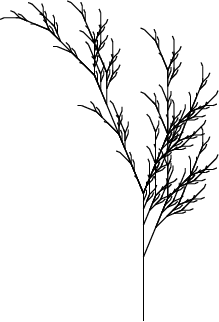
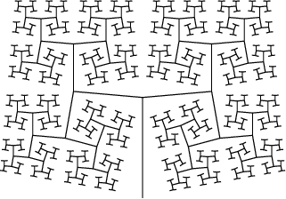
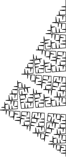
Lsystem is inspired by the book 'Algorithmic Beauty of Plants' (ABOP) by
Prusinkiewcz and Lindenmayer. Most of the systems described in the book can be
implemented with this package (and the missing features are coming soon).
Lsystem is quite general, supporting context-dependent, parameterized,
stochastic L-systems. I will write specific documentation when the feature set
is stable.
Specifying systems in Lsystem is currently a bit verbose (see the examples in
the following sections), but there are special handlers for the simplest
systems. Eventually I will write a full parser for the specification language
used in ABOP.
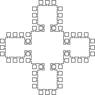
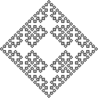
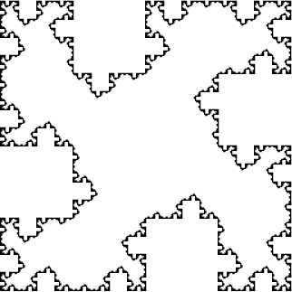
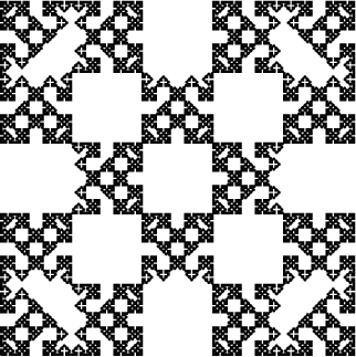
DOL-systems are deterministic, context-free, non-branching, and 2D. They can be expressed with the following 3 characters:
- 'F' - draw a line forward
- '-' - turn left
- '+' - turn right
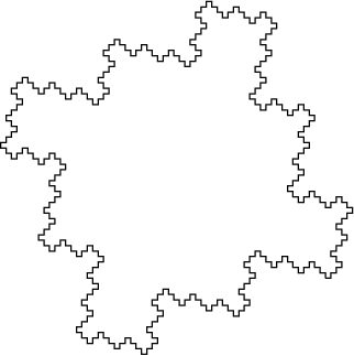
With each iteration of the system, each 'F' is replaced by a new string. In ABOP syntax, the first example below can be specified as
n=3 d=90
F-F-F-F

F -> F-F+F-F+F
where n is the number of steps to take, d is the degree of the turns,
F-F-F-F is the original string, and F -> F-F+F-F+F is a rule for replacing
F at each step. These systems can be used to generate simple fractal images.
import Lsystem
import System.Random

render' :: String -> System -> IO ()
render' = renderSystem (mkStdGen 42) (400,400)

main :: IO ()
main = do
  render' "d1.svg" $ transDolSys 3 90 "F-F-F-F" "F-F+F-F+F"
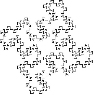
  render' "d2.svg" $ transDolSys 2 90 "F-F-F-F" "F+FF-FF-F-F+F+FF-F-F+F+FF+FF-F"
  render' "d3.svg" $ transDolSys 3 90 "F-F-F-F" "FF-F--F-F"
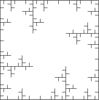
  render' "d4.svg" $ transDolSys 3 90 "F-F-F-F" "F-F-F+F+F-F-F+F+F"
  render' "d5.svg" $ transDolSys 2 90 "F-F-F-F" "FF+F+F-FFF-FFF-FFF-F+F+FF"
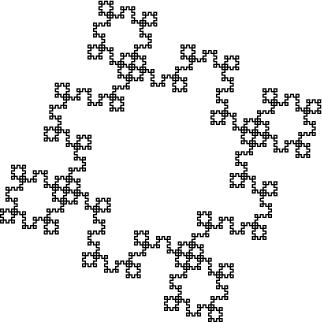
  render' "d6.svg" $ transDolSys 3 90 "F-F-F-F" "F+F+F-F-F+F-F-F+F-F-F+F+F"
  render' "d7.svg" $ transDolSys 4 90 "F-F-F-F" "FF-F+F+F-F"
  render' "d8.svg" $ transDolSys 4 90 "F-F-F-F" "FF-F-F+F+F-F+F+F-F+F+F-F-FF"
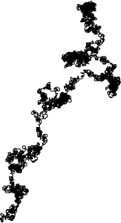
render' "d9.svg" $ transDolSys 5 90 "F" "F+F-F-F+F"L-systems can be made stochastic be adding probabilistic rules. A probabilistic rule is a set of rules associated with probabilities, where the probabilities must sum to a number less than or equal to 1 (with the implicit default rule of N -> N making up the difference).
import Lsystem
import System.Random

render' :: String -> System -> IO ()
render' = renderSystem (mkStdGen 42) (400,400)

-- Where the arguments are:
--  1. number of steps
--  2. angle
--  3. initial state
--  4. weighted list of random replacements
s1 = transSolSys 12 45 "F" [(0.4, "FF"), (0.5, "-F"), (0.1, "FF-FF-FF-FF")]

main :: IO ()
main = do
render' "s1.svg" s1I currently don't have any sugar for branching. So I will do this the hard way.
import Lsystem
import System.Random

render' :: String -> System -> IO ()
render' = renderSystem (mkStdGen 42) (400,400)

-- -- This example is taken from ABOP pp. 25
-- n=5 d=25.7
-- F -> F[+F]F[-F]F

b1 = System {
      systemBasis = [NodeDraw [] 1] -- F
    , systemRules = [               -- F[+F]F[-F]F
        DeterministicRule {
            ruleContext = ignoreContext
          , ruleCondition = unconditional
          , ruleMatch = matchF
          , ruleReplacement = constantReplacement [
                NodeDraw [] 1 ------------------ F
              , NodeBranch [[ ------------------ [+F]
                    NodeRotate [] (-25.7) 0 0
                  , NodeDraw [] 1
                ]]
              , NodeDraw [] 1 ------------------ F
              , NodeBranch [[ ------------------ [-F]
                    NodeRotate [] 25.7 0 0
                  , NodeDraw [] 1
                ]]
              , NodeDraw [] 1 ------------------ F
            ]
        }
      ]
    , systemSteps = 5
  }

main :: IO ()
main = do
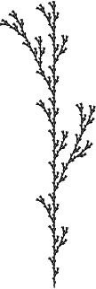
render' "b1.svg" b1Putting together the previous two examples, we can make more plant-like constructions
-- n=5 f=22.5
-- X
-- X -> F-[[X]+X]+F[+FX]-X
-- F -> FF

dummy = System {
      systemBasis = [x]
    , systemRules = [
        DeterministicRule {
            ruleContext = ignoreContext
          , ruleCondition = unconditional
          , ruleMatch = matchDummy [] "X"
          , ruleReplacement = constantReplacement [
                f, m                                   -- F-
              , NodeBranch [[NodeBranch [[x]], p, x]]  -- [[X]+X]
              , p, f                                   -- +F
              , NodeBranch [[p,f,x]]                   -- [+FX]
              , m, x                                   -- -X
            ]
        },
        DeterministicRule {
            ruleContext = ignoreContext
          , ruleCondition = unconditional
          , ruleMatch = matchF
          , ruleReplacement = constantReplacement [f,f]
        }
      ]
    , systemSteps = 5
  } where
  p = NodeRotate [] 22.5    0 0
  m = NodeRotate [] (-22.5) 0 0
  f = NodeDraw [] 1
x = NodeDummy [] "X"Some l-systems require that several variables be drawn. For example the Sierpiński arrowhead curve:
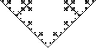
Axiom: A
Rules:
A=B-A-B
B=A+B+A
where both A and B need to be drawn
in such cases the the matchDraw can be used appropriately
thesystem = System {
    systemBasis = [NodeDraw [] 1] -- A is the axiom
    , systemRules = [

        DeterministicRule {
            ruleContext = ignoreContext
            , ruleCondition = unconditional
            , ruleMatch = matchDraw 1 -- match A
            , ruleReplacement = constantReplacement [
                b, m, a, m, b -- B-A-B
            ]
        },

        DeterministicRule {
            ruleContext = ignoreContext
            , ruleCondition = unconditional
            , ruleMatch = matchDraw 2 -- match B
            , ruleReplacement = constantReplacement [
                a, p, b, p, a
            ]
        }
    ], systemSteps = 8
} where
    a = NodeDraw [] 1 -- as decided beforehand
    b = NodeDraw [] 2 -- B, as decided beforehand
    p = NodeRotate [] 60 0 0
    m = NodeRotate [] (-60) 0 0

main :: IO ()
main = do
    render' "sierpinki_arrowhead.svg" thesystem
Summary of usage: to match nodeDraw [] 1 use matchDraw 1 for the ruleMatch and so on (the number changes for different variables)
in above example and lsystem A is NodeDraw [] 1 and was matched using matchDraw 1 and B is NodeDraw [] 2 and was matched using matchDraw 2
Note: ** Do Not use matchF when there are more than one NodeDraw that need to be matched separately **
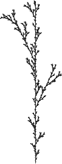
-- n=26 d=25.75
-- ignore  +-F
-- F1F1F1
--
-- 0 0 0 -> 0
-- 0 0 1 -> 1[+F1F1]
-- 0 1 0 -> 0
-- 0 1 1 -> 1
-- 1 0 0 -> 0
-- 1 0 1 -> 1F1
-- 1 1 0 -> 0
-- 1 1 1 -> 0
-- * - * -> +
-- * + * -> -

contextual = System {
      systemBasis = [f,a,f,b,f,b]
    , systemRules = [
          StochasticRule [(0.97, DeterministicRule c000          unconditional isA [b]                              )] -- 0 0 0 -> 1
        , StochasticRule [(0.97, DeterministicRule c001          unconditional isA [a]                              )] -- 0 0 1 -> 0
        , StochasticRule [(0.97, DeterministicRule c010          unconditional isB [a]                              )] -- 0 1 0 -> 0
        , StochasticRule [(0.97, DeterministicRule c011          unconditional isB [b,f,b]                          )] -- 0 1 1 -> 1F1
        , StochasticRule [(0.97, DeterministicRule c100          unconditional isA [b]                              )] -- 1 0 0 -> 1
        , StochasticRule [(0.97, DeterministicRule c101          unconditional isA [b, NodeBranch [[ p,f,b,f,b ]]]  )] -- 1 0 1 -> 1[+F1F1]
        , StochasticRule [(0.97, DeterministicRule c110          unconditional isB [b]                              )] -- 1 1 0 -> 1
        , StochasticRule [(1.00, DeterministicRule c111          unconditional isB [a]                              )] -- 1 1 1 -> 0
        , StochasticRule [(0.97, DeterministicRule ignoreContext unconditional isP [m]                              )] -- * - * -> +
        , StochasticRule [(0.98, DeterministicRule ignoreContext unconditional isM [p]                              )] -- * + * -> -
      ]
    , systemSteps = 27
  } where

  f = NodeDraw [] 1
  a = NodeDummy [] "0"
  b = NodeDummy [] "1"
  p = NodeRotate []   25.75  0 0
  m = NodeRotate [] (-25.75) 0 0

  ss = [p,m,f]

  isA = matchDummy [] "0"
  isB = matchDummy [] "1"

  isP :: Node -> a -> Maybe a
  isP (NodeRotate _ a _ _) x | a > 0 = Just x
                             | otherwise = Nothing
  isP _ _ = Nothing

  isM :: Node -> a -> Maybe a
  isM (NodeRotate _ a _ _) x | a < 0 = Just x
                             | otherwise = Nothing
  isM _ _ = Nothing

  c000 = contextMatch ss [a] [a]
  c001 = contextMatch ss [a] [b]
  c010 = contextMatch ss [a] [a]
  c011 = contextMatch ss [a] [b]
  c100 = contextMatch ss [b] [a]
  c101 = contextMatch ss [b] [b]
  c110 = contextMatch ss [b] [a]
c111 = contextMatch ss [b] [b] The replacement string is a function of the original symbol and the context. Each symbol holds a vector of doubles, which can be used pass extra information. This example comes from ABOP pp. 47.
par1 = System {
      systemBasis = basis
    , systemRules = [
        DeterministicRule {
              ruleContext     = ignoreContext
            , ruleCondition   = unconditional
            , ruleMatch       = matchDummy "A"
            , ruleReplacement = r_repl
          }
      ]
    , systemSteps = 10
  } where

  r = 1.456

  p = NodeRotate []   85  0 0
  m = NodeRotate [] (-85) 0 0

  -- A(1)
  basis = [NodeDummy [1] "A"]

  -- F(s)[+A(s/R)][-A(s/R)]
  r_repl _ _ (NodeDummy [s] _) = [
         NodeDraw [] s                          -- F(s)
      ,  NodeBranch [
             [p, NodeDummy [s/r] "A"]  -- [+A(s/R)]
           , [m, NodeDummy [s/r] "A"]  -- [-A(s/R)]
         ]
    ]
#define c 1.0
#define p 0.3
#define q c - p
#define h sqrt (p * q)
w : f(0,1)
p1 : F(x,t) : t = 0 : F(x*p, 2) + F(x*h, 1) -- F(x*h, 1) + F(x*q, 0)
p2 : F(x,t) : t > 0 : F(x, t-1)
par2 = System {
      systemBasis = basis
    , systemRules = [
          DeterministicRule {
                ruleContext     = ignoreContext
              , ruleCondition   = r1_cond
              , ruleMatch       = isF
              , ruleReplacement = r1_repl
            }
        , DeterministicRule {
                ruleContext     = ignoreContext
              , ruleCondition   = r2_cond
              , ruleMatch       = isF
              , ruleReplacement = r2_repl
            }
      ]
    , systemSteps = 8
  } where

  c = 1.0
  p = 0.3
  q = c - p
  h = sqrt (p * q)

  p' = NodeRotate []   86  0 0
  m' = NodeRotate [] (-86) 0 0

  -- f(0,1)
  basis = [NodeDraw [0] 1]

  -- t = 1
  r1_cond _ _ (NodeDraw [t] _) x
    | t == 0 = Just x
    | otherwise = Nothing
  r1_cond _ _ _ _ = Nothing

  -- F(x*p, 2) + F(x*h, 1) - - F(x*h, 1) + F(x*q, 0)
  r1_repl _ _ (NodeDraw [t] x) = [
         NodeDraw [2] (x*p) -- F(x*p, 2)
       , p'                 -- +
       , NodeDraw [1] (x*h) -- F(x*h, 1)
       , m'                 -- -
       , m'                 -- -
       , NodeDraw [1] (x*h) -- F(x*h, 1)
       , p'                 -- +
       , NodeDraw [0] (x*q) -- F(x*q, 0)
    ]

  -- t > 0
  r2_cond _ _ (NodeDraw [t] _) x
    | t > 0 = Just x
    | otherwise = Nothing
  r2_cond _ _ _ _ = Nothing

  -- F(x, t-1)
  r2_repl _ _ (NodeDraw [t] x) = [ NodeDraw [t-1] x ]
Modeling realistic trees requires two new features: variation in line width and 3-dimensional systems. This example is taken from ABOP pp. 60.
#define d1 94.74     /* divergence angle 1  */
#define d2 132.62    /* divergence angle 2  */
#define a  18.95     /* branching angle     */
#define lr 1.109     /* elongation rate     */
#define vr 1.732     /* width increase rate */

w = !(1)F(200)/(45)A
A    : * -> !(vr )F(50)[&(a)F(50)A]/(d1)
            [&(a)F(50)A]/(d2)[&(a)F(50)A]
F(l) : * -> F(l*lr )
!(w) : * -> !(w*vr )
- deterministic
- stochastic
- branching
- dummy variables
- context sensitive
- parametric
- stochastic sugar
- deterministic sugar
- branching sugar
- parametric sugar
- context sensitive sugar
- 2D visualization
- 3D handling
- 3D visualization
- animation
- polygons
- colors and such
- ABOP language parsing
