Zalando Classification Task

Problem Description

We’re given a dataset with the following properties:

Size: 1,000,000 (1 million) datapoints
Dimensionality: 100
Classes: 2 (binary classification)
Balance: Perfectly balanced (50% positive, 50% negative)

Hints

We’re told that the optimal classifier is around 90% accurate. This is possible to know if one has access to the underlying data generating process and can compute the densities P(x | y=1) and P(x | y=0). The Bayes optimal classifier is then given by P(y=1|x) = P(x | y=1) / [P(x | y=1) + P(x | y=0)] (see https://tiao.io/post/density-ratio-estimation-for-kl-divergence-minimization-between-implicit-distributions/ for an example derivation).
We’re also told that the features are highly-dependent.

Approach

Before diving into any sophisticated techniques, it’s always a good idea to try out some naive methods to use as a baseline, like Naive Bayes (NB) or k-Nearest Neighbors (k-NN). Thereafter, it’s reasonable to attack the problem with popular methods that have consistently dominated in data science competitions like Kaggle. Some of these include ensemble methods like Random Forests and Gradient Boosting (XGBoost). Some other promising approaches include Multi-layer Perceptrons (MLPs), Support Vector Classification (SVC) and Gaussian Process Classification (GPC).

Preliminary results

For model evaluation, we first created a hold-out test set consisting of 20% of the datapoints we were given. With the naive baselines (NB, k-NN), we hovered around 50% test accuracy.

In preliminary analysis (without making significant effort to tune the model hyperparameters), we consistently obtained at best around 55% test accuracy with Random Forests, Gradient Boosting and SVC.

In the last model (GPC), exact posterior inference is not tractable, especially given with size of the dataset. While approximate methods are available, it is left outside the scope of this solution set. I felt it deserved a special mention nonetheless since it particularly well-suited to this problem — it is capable of capturing complex dependencies between features (which is important according to Hint 2), and comes with a principled approach to feature selection when Automatic Relevance Determination (ARD) kernels are used.

Multi-layer Perceptron

We obtained decent results with Multi-layer Perceptions (MLPs). In particular, we considered a simple family of MLPs with "rectangular shapes" (number of hidden units are constant across all hidden layers). We primarily experimented with 2 hidden layers each with 64 hidden units, and ReLU activations.

We assessed our model with k-fold cross-validation. Since each model takes approximately 20 mins to train for 50 epochs, and we need to train a separate model for each fold, we limit k to a modest value of k=3.

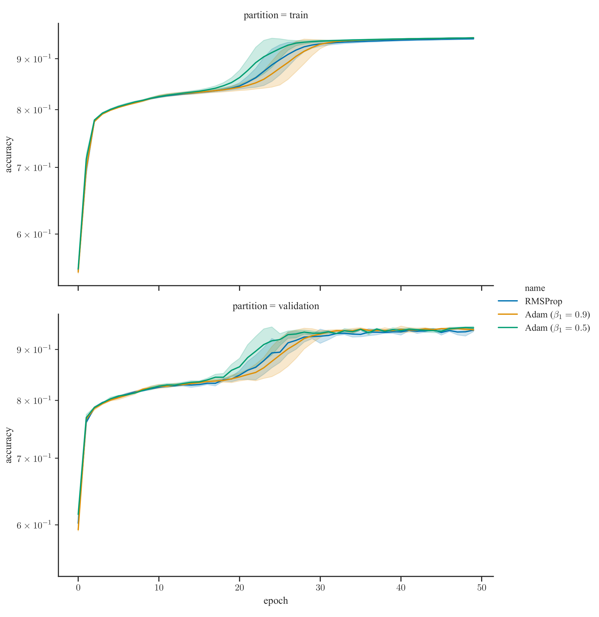
Across cross-validation folds, with slight variations on hyperparameters such as optimizer parameters, we were able to consistently achieve a validation accuracy of around 94% as shown in the learning curve plots below. The hue represents different optimizers/parameters; the top row shows the train accuracy over epochs while the bottom row shows the validation accuracy; the solid lines denotes the mean accuracy across folds while the shaded error bands denotes the standard deviation.

While varying the optimizers and their parameters didn't have a significant impact on final performance (all eventually converge to around 94%), some settings resulted in faster convergence than others. In particular, one can observe that Adam with beta1=0.5 converges faster than RMSProp, which in turn converges faster than Adam with beta1=0.9 (the default in practically all deep learning libraries).

We also experimented with different data pre-processing methods such as normalization and whitening (standardization), but these mostly had deleterious effects on performance. The same was true for regularization methods such as weight decay and Dropout, and also for layer normalization techniques such as Batch normalization, which worsened performance by as much as 10%.

Usage

Clone this repository:

$ git clone https://github.com/ltiao/zalando-classification.git

The datasets are tracked using text pointers with Git Large File Storage (LFS). It is recommended that this be installed prior to cloning.

Getting started

The quickest way to get started is by running the Docker container with Docker image tiao/zalando-classification:

$ docker run -it --rm tiao/zalando-classification zalando_classification --help
Usage: zalando_classification [OPTIONS] NAME

Options:
  --optimizer TEXT
  -e, --epochs INTEGER            Number of epochs.
  -b, --batch-size INTEGER        Batch size.
  --evaluate-only                 Skip model fitting. Only evaluate model.
  --resume-from-epoch INTEGER     Epoch at which to resume a previous training
                                  run
  --l1-factor FLOAT               L1 regularization factor.
  --l2-factor FLOAT               L2 regularization factor.
  --batch-norm / --no-batch-norm  Use Batch Normalization (after activation).
  --standardize
  --split-method [kfold|shuffle]  Method for generating train/test dataset
                                  splits.
  --n-splits INTEGER              Number of train/test dataset splits.
  --test-size FLOAT               Test set size (for shuffle split method
                                  only).
  --checkpoint-dir DIRECTORY      Model checkpoint directory.
  --checkpoint-period INTEGER     Interval (number of epochs) between
                                  checkpoints.
  --summary-dir DIRECTORY         Summary directory.
  -s, --seed INTEGER              Random seed
  --help                          Show this message and exit.

GPU Support

Use Nvidia Container Toolkit to run with Nvidia GPU Support. Append option --gpus all to the docker run command.

Reproducing results from pre-trained model

To reproduce results with pre-trained model, run the following (from the directory containing the datasets/ and models/ directories):

$ docker run --gpus all -it --rm -v "$PWD/datasets":/usr/src/app/datasets -v "$PWD/models":/usr/src/app/models tiao/zalando-classification zalando_classification --seed=8888 --split-method=kfold --n-splits=3 --evaluate-only --resume-from-epoch=50 rmsprop
333334/333334 [==============================] - 9s 26us/sample - loss: 0.1589 - acc: 0.9450
[Split 0] test accuracy: 0.945, test loss 0.159
333333/333333 [==============================] - 8s 23us/sample - loss: 0.1727 - acc: 0.9387
[Split 1] test accuracy: 0.939, test loss 0.173
333333/333333 [==============================] - 8s 24us/sample - loss: 0.1697 - acc: 0.9398
[Split 2] test accuracy: 0.940, test loss 0.170

Train model from scratch

To train new models from scratch:

$ docker run -it --rm --gpus all -v "$PWD/datasets":/usr/src/app/datasets -v "$PWD/models":/usr/src/app/models -v "/logs":/usr/src/app/logs tiao/zalando-classification zalando_classification --seed=8888 --split-method=kfold --n-splits=3 new

You can find model checkpoints in $PWD/models, logs of losses and metrics in $PWD/logs, both in CSV format and as TensorBoard Summaries. In another terminal window, you can launch TensorBoard at the appropriate log directory, e.g.

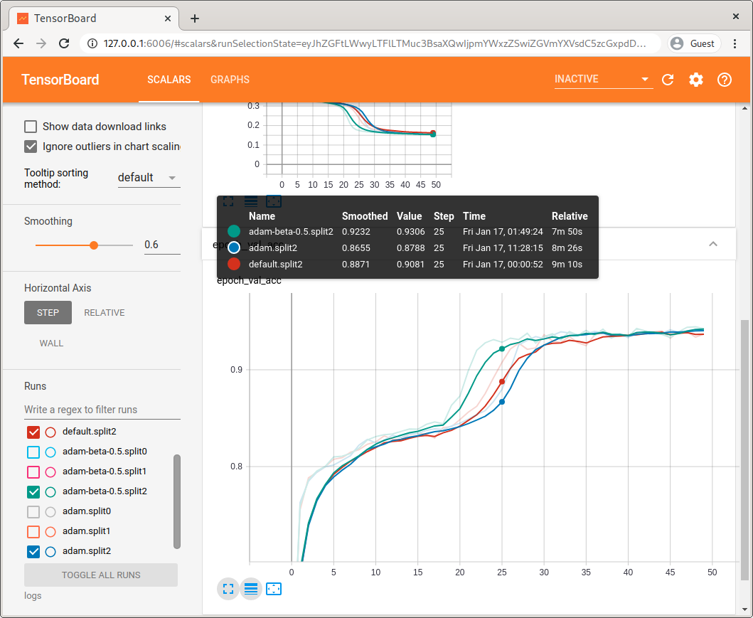
$ tensorboard --logdir=$PWd/logs

Navigate to http://127.0.0.1:6006/ in your browser to see live training summaries updated in real-time:

Compile documentation

To compile documentation (which generates the learning curve plots shown above):

$ docker run -it --rm -v "$PWD/docs":/usr/src/app/docs -v "$PWD/logs":/usr/src/app/logs tiao/zalando-classification make docs

Docker Build

To build the image from scratch:

$ make docker-build

Credits

The boilerplate for this package was created with Cookiecutter and the audreyr/cookiecutter-pypackage project template.

ltiao / zalando-classification