litaotao / machine-learning-crash-course

machine-learning-crash-course from google

machine-learning-crash-course

machine-learning-crash-course from google

Introduction to Machine Learning

Learning Objectives

Recognize the practical benefits of mastering machine learning

Understand the philosophy behind machine learning

• machine learning can help us solve problems more efficiently and make it possible to answer questions that can not be answered before;
• the concept behind machine learning can help us build a more complicated and sound and logical mind when facing other problems;

Framing

This module investigates how to frame a task as a machine learning problem, and covers many of the basic vocabulary terms shared across a wide range of machine learning (ML) methods.

Learning Objectives

• Refresh the fundamental machine learning terms.
• Explore various uses of machine learning.

• supervised ML

  Supervised ML models use the input to produce useful predictions on never-before-seen data;

  When train supervised ML, we need feed the model with labels(y) and features(x), example(实例) is a particular instance of data, labeled example has {features, label}, that's (x, y), used to train the model, unlabeled example has {features, ?}, that's (x, ?), used for making predictions.

  And the model is something that maps examples to predicted labels (y'), defined by internal parameters, which are learned (where the word "machine learning" comes from).

• Key ML Terminology

  • supervised ML: ML systems learn how to combine input to produce useful predictions on never-before-seen data;
  • Labels: A label is the thing we're predicting - the y variable in simple linear regression.
  • Features: a feature is an input variable - the x variable in simple linear regression, a simple ML might use a single feature, while a more sophisticated ML could use millions of features, specified as $\left{ x_1, x_2, … , x_n \right}$, in the spam detector example, the features could include the following:
    • words in the email text
    • sender's address
    • time of day the email was sent
    • Email contains the phrase "one weird trick"
  • Training: means creating or learning the model, that is you show the model labeled examples and enable the model to gradually learn th relationships between features and labels;
  • inference: means applying the trained model to unlabeled examples, that is use the trained model to make useful predictions (y').
  • Regression: a regression model predicts continuous values;
  • Classification: a classification model predicts discrete values;

Descending into ML

Linear regression is a method for finding the straight line or hyperplane that best fits a set of points.

Learning Objectives

• Refresh your memory on line fitting.
• Relate weights and biases in machine learning to slope and offset in line fitting.
• Understand "loss" in general and squared loss in particular.

we use loss to evaluate the performance of our trained models, the most common loss is $L_2 Loss ( also \ known \ as \ squared \ loss)$ as bellow: $$ L_2 Loss = \sum_{(x, y)} (y - prediction(x)){}^{2} = \sum (y - y'){}^2 $$

$$ MSE = Mean \ Square \ Error = \frac 1 N \sum_{(x, y)} (y - y')_{}^2 $$

training a model simply means learning good values for all the weights and the bias from labeled examples. in supervised learning, a machine learning algorithm builds a model by examining many examples and attempting to find a model that minimize loss, this process is called empirical risk minimization.

loss is the penalty for a bad prediction, that is loss is a number indicating how bad [[the model's predictions was on a single example.

Although MES is commonly-used in machine learning, it's neither the only practical loss function nor the best loss function for all circumstances.

Reducing loss

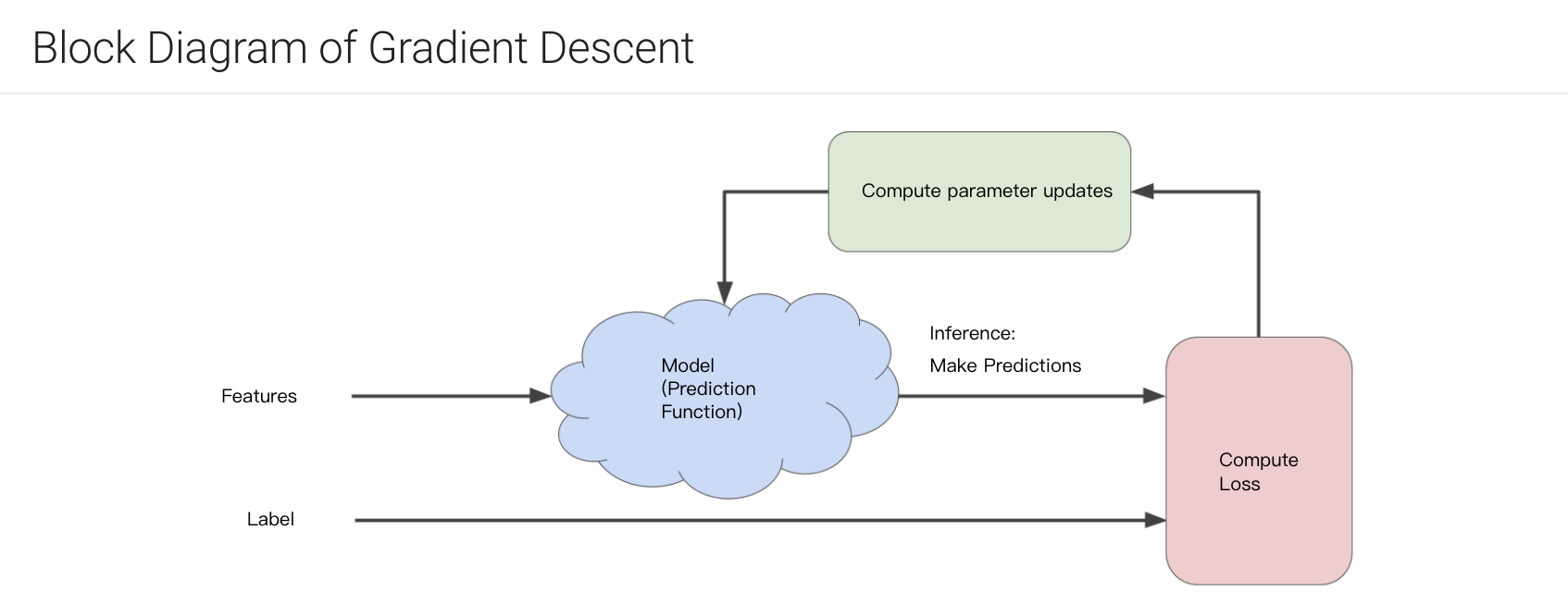
• gradient decent

  

• Weight initialize

For convex (like of a bowl shape) problems, weights can start anywhere (say, all 0's), for there is just one minimum.

For non-convex problems (like of an egg crate), there exists more than one minimum, the final results strongly depend on the initial values of weights.

• SGD & Mini-Batch Gradient Descent

We could compute gradient over entire data set on each step, but this turns out to be unnecessary and less efficient, a gradient is a vector of partial derivatives;

Problem: what is the gradient vector of model: $y = wx + b$.

We can compute gradient on small data set, for example, we get a new random sample on every step;

• Sthochastic Gradient Descent: one example at a time, and the term stochastic indicates that the one example comprising each batch is chosen at random;
• Mini-Batch Gradient Descent: we get a small data sample (10-1000 examples) every time, in this way, the loss and gradients are averaged over the batch, which would be more stable;

• learning rate

The gradient vector has both a direction and a magnitude, gradient descent algorithms multiply the gradient by a scalar known as the learning rate ( also sometimes called step size ) to determine the next point.

hyperparamters are the knobs or paramters that programmers set and tweak in machine learning algorithms, learning rate is kind of a hyper parameters.

the ideal learning rate in one-dimension is $\frac 1 {f(x)_{}^{''}}$, that's the inverse of the second derivative of f(x) as x;

the ideal learning rate in 2-dimension or more dimensions is the inverse of the hessian, that is matrix of second partial derivative;

First Steps with TF

Learning Objectives

• Learn how to create and modify tensors in TensorFlow.
• Learn the basics of pandas.
• Develop linear regression code with one of TensorFlow's high-level APIs.
• Experiment with learning rate.

TF consists of the following two components:

• a graph protocol buffer
• a runtime that executes the (distributed) graph

These two components are analogous to the java compiler and the JVM, just as the JVM is implemented on multiple hardware platforms, so is TF-CPUs and TF-GPUs.

• Common hyperparameters in TF
  • steps: total number of training iterations, one step calculates the loss from one batch and uses that value to modify the model's weights once;
  • batch size: which is the number of examples (chosen at random) for a single step, for example the batch size for SGD is 1;
  • periods: the granularity of reporting, modifying periods does not alter what your model learns.

$$ total \ number \ of \ trained \ examples = batch \ size * steps $$

$$ number \ of \ training \ examples \ in \ each \ period = \frac {batch \ size * steps} {periods} $$

Generalization

generalization refers to your model's ability to adapt properly to new, previously unseen data, drawn from the same distribution as the one used to create the model.

the fundamental tension of machine learning is between fitting our data well, but also fitting the data as simply as possible.

the following 3 basic assumptions guide generalization:

• we draw examples independently and identically at random from the distribution, in other words, examples don't influence each other;
• the distribution is stationary, that's the distribution doesn't change within the data set;
• we draw examples from partitions from the same distribution;

In practice, we sometimes violate these assumptions, for example:

• consider a model that chooses ads to display, the iid assumption would be violated if the model bases its choice of ads, in part, on what ads the user has previously seen;
• consider a data set that contains retail sales information for a year, user's purchase change seasonally, which would violate stationarity;

Training and Test Sets

a test set is a data set used to evaluate the model developed from a training set.

Make sure that your test set meets the following 2 conditions:

• is large enough to yield statistically meaningful results;
• is representative of the data set as a whole, in other words, don't pick a test set with different characteristics than the training set;

Validation: Check Your Intuition

partitioning a data set into a training set and test set lets you judge whether a given model will generalize well to new data. However, using only two partitions maybe insufficient when doing many rounds of hyperparameter tuning. we need a validation set in a partitioning shcema

so the best work flow for training:

• Pick the model that does best on the validation set
• Double-check that model against the test set

this is a better workflow because it creates fewer exposures to the test set.

Representation

A machine learning model can't directly see, hear or sense input examples. Instead you must create a representation of the data to provide the model with a useful vantage point into the data's key qualities. that is, in order to train a model, you must choose the set of features that best represent the data.

Learning Objectives

• Map fields from logs and protocol buffers into useful ML features.
• Determine which qualities comprise great features.
• Handle outlier features.
• Investigate the statistical properties of a data set.
• Train and evaluate a model with tf.estimator.

the following are about cleaning data.

• scaling feature values:

  scaling means converting floating-point feature values from their natural range into a standard range (for example, 0 to 1 or -1 to +1). if a feature set consists of only a single feature, then scaling provides little to no practical benefit. If, however, a feature set consists of multiple features, then feature scaling provides the following benefits:

  • helps gradient descent converge more quickly;
  • Helps avoid the "nan trap", in which one number in the model becomes a nan and due-to math operations-every other number in the model also eventually becomes a nan;
  • helps the model learn appropriate weights for each feature, without feature scaling, the model will pay too much attention to the features having a wider range;

• handling extreme outliers:

  • Apply log function on the features
  • If still exists outliers, use cap way.

• binning:

  that is do not use the raw values of a feature, but map the raw value to a discrete group, and use the group number as the feature values. just something like quantile method.

• scrubbing:

  in real-life, many examples in data sets are unreliable due to one or more of the following:

  • omitted values:
  • duplicate examples:
  • bad labels:
  • bad feature values:

Feature Crosses

A feature cross is a synthetic feature formed by multiplying (crossing) two or more features, crossing combinations of features can provide predictive abilities beyond what those features can provide individually.

Learning Objectives

• Build an understanding of feature crosses.
• Implement feature crosses in TensorFlow.

Regularization for Simplicity: Playground Exercise

regularization means penalizing the complexity of a model to reduce overfitting.

The generalization curve shows the loss for both the training set and validation set against the number of training iterations.

The model's generalization curve above means that the model is overfitting to the data in the training set. This may be caused by a complex model, we use regularization to prevent overfitting, traditional way, we optimize a model by find the minimize loss, as bellow formula show: $$ minimize(Loss(data | model)) $$ But this would not consider the complexity of the model, so we use a so-called structural risk minimization way to optimize a model: $$ minimize(Loss(data | model) + complexity(model)) $$

• the loss term: measures how well the model fits the data
• the regularization term: measures the model's complexity

this course focuses on two common ways to think of model complexity:

• model complexity as a function of the weights of all the features in the model
• model complexity as a function of the total number of features with nonzero weights

We can quantify complexity using the L2-regularization formula, which defines the regularization term as the sum of the squares of all the feature weights: $$ L2 \ regularization \ term = ||w||_{2}^{2} = w_1^2 + w_2^2 + ... + w_n^2 $$ Practically, model developers tune the overall impact of the regularization term by multiplying its value by a scalar known as lambda (or the regularization rate), that's the formula bellow: $$ minimize(Loss(data | model) + \lambda * complexity(model)) $$ performing L2 regularization has the following effect on a model:

• encourages weight values toward 0
• encourages the mean of the weights toward 0, with a normal (bell-shaped or Gaussian) distribution

Increasing the lambda value strengthens the regularization effect, for example, the histogram of weights for a high value of lambda might look as bellow:

lowering the value of lambda tends to yield a flatter histogram, like bellow:

When choosing a lambda value, the goal is to strike the right balance between simplicity and a training-data fit:

• if your lambda value is too high, your model will be simple, but you run the risk of underfitting your data, your model won't learn enough about the training data to make useful predictions;
• if your lambda value is too low, your model will be more complex, and you run the risk of overfitting your data, your model will learn too much about the particularities of the training data, and won't be able to generalize to new data;

there's a close connection between learning rate and lambda, strong L2 regularization values tend to driver feature weights closer to 0. Lower learning rates(with early stopping) often produce the same effect because the steps away from 0 aren't as large. Consequently, tweaking learning rate and lambda simultaneously may have confounding effects.

early stopping means ending training before the model fully reaches convergence. in practice, we often end up with some amount of implicit early stopping when training in an online fashion. that's some new trends just haven't had enough data yet to converge.

the effects from changes to regularization parameters can be confounded with the effects from changes in learning rate or number of iterations. one useful practice is to give yourself a high enough number of iterations that early stopping doesn't play into things.

Logistic Regression

instead of predicting exactly 0 or 1, logistic regression generates a probability —— a value between 0 and 1.

Learning Objectives

• Understand logistic regression.
• Explore loss and regularization functions for logistic regression.

Many problems require a probability estimate as output, logistic regression is an extremely efficient mechanism for calculating probabilities. in many cases, you'll map the logistic regression output into the solution to a binary classification problem, in which the goal is to correctly predict one of two possible labels. you might be wondering how a logistic regression model can ensure output that always falls between 0 and 1. a sigmoid function defined as follows, produces output having those same characteristics: $$ y = \frac 1 {1 + e_{}^{-x}} $$

if x represents the output of the linear layer of a model trained with logistic regression, the sigmoid(x) will yield a probability between 0 and 1.

the loss function for linear regression is squared loss, the loss function for logistic regression is log loss, which is defined as follows: $$ LogLoss = \sum_{x, y} -y * log(y') - (1-y) * log(1 - y') $$

• y is the label in a labeled example, since this is logistic regression, every value of y must either be 0 or 1;
• y' is the predicted value(somewhere between 0 and 1), given the set of features in x;

Classification

this module shows how logistic regression can be used for classification tasks, and explores how to evaluate the effectiveness of classificatin models.

Learning Objectives

• Evaluating the accuracy and precision of a logistic regression model.
• Understanding ROC Curves and AUCs.

Logistic regression returns a probability. you can use the returned probability directly or convert the returned probability to a binary value.

$$ accuracy = \frac {TP + TN}{TP + TN + FP + FN} $$ Sometimes use accuracy may ignore some detail and import problem on the model it self, here is an example bellow:

in the photo above, the accuracy of this model is (1 + 90) / (1 + 90 + 1 + 8) = 0.91. which seems great. But let's do a closer analysis of positives and negatives to gain more insight into our model's performance:

• Of the 100 tumor examples, 91 are benign (90 TN and 1 FP) and 9 are maligant(1 TP and 8 FN)
• of the 91 benign tumors, the model correctly identifies 90 as benign, that's great; however, of the 9 malignant tumors, the model only correctly identifies 1 as malignant - a terrible outcome, as 8 out of 9 malignancies go undiagnosed.

while 91% accuracy may seem good at first glance, another tumor-classifier model that always predicts benign would achieve the exact same accuracy (0.91) on our example. in other words, our model is no better than one that has zero predictive ability to distinguish malignant tumors from benign tumors.

Accuracy alone doesn't tell the full story when you're working with a class-imbalanced data set, like this one, where there is a significant disparity between the number of positive and negative labels.

so we derived some other evaluate method to value a model.

precision answer the question what proportion of positive identifications was actually correct?, and is defined as follows: $$ precision = \frac {TP}{TP + FP} $$ in the above model, the precision is (1)/(1 + 1) = 50%，our model has a precision of 0.5, in other words, when it predicts a tumor is malignant, it is correct 50% of the time.

recall answer the question what proportion of actual positives was identified correctly, is defined as follows: $$ recall = \frac {TP}{TP + FN} $$ our model has a recall of (1)/(1+8) = 0.11, in other words, it correctly identifies 11% of all malignant tumors.

to fully evaluate the effectiveness of a model, you must examine both precision and recall. But precision and recall are often in tension, that's improving precision typically reduces recall and vice versa. so sometimes we use F1 score to evaluate a model, which rely on both precision and recall.

Besides precision, recall and F1 score, we also have 2 powerful tool to evaluate a model, that's ROC curve and AUC.

An ROC curve (receiver operating characteristic curve) is a graph showing the performance of a classification model at all classification thresholds. this curve plots two parameters:

• True Positive Rate
• False Positive Rate

True positive rate(TPR) is a synonym for recall and is therefore defined as follows: $$ TPR = \frac {TP}{TP + FN} $$ False positive rate(FPR) is defined as follows: $$ FPR = \frac {FP}{FP + TN} $$ an roc curve plots TPR vs FPR at different classification thresholds. lowering the classification threshold classifies more items as positive, thus increasing both FP and TP, the following figure shows a typical ROC curve:

to compute the points in an ROC curve, we could evaluate a logistic regression model many times with different classification thresholds, but this would be inefficient. But there'is an efficient and sorting-based algorithm that can provide this information for us, called AUC.

AUC stands for area under the ROC curve, that's measures the entire two-dimensional area underneath the entire ROC curve from (0, 0) to (1, 1).

AUC provides an aggregate measure of performance across all possible classification thresholds. One way of interpreting AUC is as the probability that the model ranks a random positive example more highly than a random negative example.

for more information, check bellow:

• 精确率、召回率、F1 值、ROC、AUC 各自的优缺点是什么？

logistic regression predictions should be unbiased, that's average of predictions should equal to average of observations, and prediction bias is a quantity that measures how far apart those two averages are, that is: $$ prediction \ bias = average \ of \ predictions - average \ of \ labels \ in \ data \ set $$ A significant nonzero prediction bias tells you there is a bug somewhere in your model, as it indicates that the model is wrong about how frequently positive labels occur.

For example, let's say we know that on average, 1% of all emails are spam. If we don't know anything at all about a given email, we should predict that it's 1% likely to be spam. Similarly, a good spam model should predict on average that emails are 1% likely to be spam. (In other words, if we average the predicted likelihoods of each individual email being spam, the result should be 1%.) If instead, the model's average prediction is 20% likelihood of being spam, we can conclude that it exhibits prediction bias.

possible root causes of prediction bias are:

• Imcomplete feature set
• noisy data set
• buggy pipeline
• Biased training sample
• overly strong regularization

Regularization for Sparsity