areal

Areal interpolation is the process making estimates from a source set of polygons to an overlapping but incongruent set of target polygons. One challenge with areal interpolation is that, while the processes themselves are well documented in the academic literature, implementing them often involves “reinventing the wheel” by re-creating the process in the analyst’s tool choice.

While the R package sf does offer a basic interface for areal weighted interpolation (st_interpolate_aw), it lacks some features that we use in our work. The areal package contains a suite tools for validation and estimation, providing a full-featured workflow that fits into both modern data management (e.g. tidyverse) and spatial data (e.g. sf) frameworks.

Bug Fixes in v0.1.4

There are two additional bug fixes in v0.1.4:

Data that do not require being converted back from a geometry collection (see #2 in the next section) were still being processed through this code, making runtimes longer than necessary. This has been fixed.
Mixed interpolations with multiple extensive and intensive variables would get incorrect output containing two copies of the extensive results. This has been fixed, and the simplest workaround is to install the development version of areal from GitHub.

Bug Fixes in v0.1.3

The initial CRAN release contains four known bugs (see Issues 6, 7, 14, and 16), all of which are fixed on the current GitHub master branch:

If the tid and sid column names are identical, the interpolated column created by aw_interpolate() will consist of all NA values. The simplest workaround is to rename either tid or sid before executing aw_interpolate(). Alternatively, you can install the development version of areal from GitHub.
Some intersections of sf geometries will result in geometry collections being created. This appears to be an infrequent issue, but it will result in an error when aw_interpolate() is executed. The error will begin with Warning in st_cast.GEOMETRYCOLLECTION(X[[i]], ...). The simplest workaround is to install the development version of areal from GitHub.
Interpolation fails if the sf geometry column is not named geometry. The simplest workaround is to either rename the column to geometry before executing aw_interpolate(). Alternatively, you can install the development version of areal from GitHub.
Interpolation with output = "tibble" only returns the identification number and the estimated value. If you want other variables from the target data, the simplest workaround is to join the output to the original target data. Alternatively, you can install the development version of areal from GitHub.

Big thanks to early adopter Matt Herman for catching the first two and David Blodgett for catching the third!

Installation

Installing Dependencies

You should check the sf package website and the areal package website for the latest details on installing dependencies for that package. Instructions vary significantly by operating system. For best results, have sf installed before you install areal. Other dependencies, like dplyr, will be installed automatically with areal if they are not already present.

The one exception here is the dependency lwgeom, which Linux users will need to follow some special instructions to install correctly.

Installing areal

The easiest way to get areal is to install it from CRAN:

install.packages("areal")

The development version of areal can be accessed from GitHub with remotes:

# install.packages("remotes")
remotes::install_github("slu-openGIS/areal")

Usage

Two function prefixes are used in areal to allow users to take advantage of RStudio’s auto complete functionality:

ar_ - data and functions that are used for multiple interpolation methods
aw_ - functions that are used specifically for areal weighted interpolation

Data

The package contains four overlapping data sets:

ar_stl_race (2017 ACS demographic counts at the census tract level; n = 106)
ar_stl_asthma (2017 asthma rates at the census tract level; n = 106)
ar_stl_wards (the 2010 political subdivisions in St. Louis; n = 28).
ar_stl_wardsClipped (the 2010 political subdivisions in St. Louis clipped to the Mississippi River shoreline; n = 28).

These can be used to illustrate the core functionality of the package. The following examples assume:

> library(areal)
>
> race <- ar_stl_race
> asthma <- ar_stl_asthma
> wards <- ar_stl_wards

Areal Weighted Interpolation

areal currently implements an approach to interpolation known as areal weighted interpolation. It is arguably the simplest and most common approach to areal interpolation, though it does have some drawbacks (see the areal weighted interpolation vignette for details). The basic usage of areal is through the aw_interpolate() function. This is a pipe-able function that allows for the simultaneous interpolation of multiple values.

In this first example, the total estimated population (TOTAL_E) of each ward is calculated from its overlapping census tracts:

aw_interpolate(wards, tid = WARD, source = race, sid = "GEOID", 
               weight = "sum", output = "sf", extensive = "TOTAL_E")
#> Simple feature collection with 28 features and 4 fields
#> geometry type:  POLYGON
#> dimension:      XY
#> bbox:           xmin: 733361.8 ymin: 4268336 xmax: 746157.7 ymax: 4295504
#> epsg (SRID):    26915
#> proj4string:    +proj=utm +zone=15 +ellps=GRS80 +towgs84=0,0,0,0,0,0,0 +units=m +no_defs
#> First 10 features:
#>    OBJECTID WARD      AREA   TOTAL_E                       geometry
#> 1         1    1  46138761  7991.565 POLYGON ((740184.2 4286431,...
#> 2         2    2 267817711 12145.021 POLYGON ((742392.1 4289178,...
#> 3         3    3  66291644  7344.287 POLYGON ((742956.1 4284113,...
#> 4         4    4  53210707  8457.672 POLYGON ((739557.6 4284080,...
#> 5         5    5  60462396  8783.377 POLYGON ((744883.8 4281632,...
#> 6         6    6  64337271 14050.399 POLYGON ((742501.6 4279976,...
#> 7         7    7 101268146 15840.086 POLYGON ((745618.6 4279867,...
#> 8         8    8  45966410 12188.131 POLYGON ((739842.8 4277724,...
#> 9         9    9  73993891 14217.149 POLYGON ((742619.4 4276734,...
#> 10       10   10  62915358 11239.213 POLYGON ((737257.7 4277050,...

This example outputs a simple features (sf) object and uses one of two options for calculating weights. All of these arguments are documented both within the package (use ?aw_interpolate) and on the package’s website.

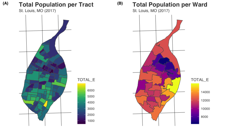
What results from aw_interpolate() is mapped below. Total population per census tract in St. Louis is mapped on the left in panel A. Using aw_interpolate() as we did in the previous example, we estimate population counts for Wards in St. Louis from those census tract values. These estimated values are mapped on the right in panel B.

Both extensive and intensive data can be interpolated simultaneously by using both the extensive and intensive arguments. In this second example, the asthma and race data are combined, and estimates for both the population values and asthma rates are calculated for each ward from its overlapping census tracts:

# remove sf geometry
st_geometry(race) <- NULL

# create combined data
race %>%
  select(GEOID, TOTAL_E, WHITE_E, BLACK_E) %>%
  left_join(asthma, ., by = "GEOID") -> combinedData

# interpolate
wards %>%
  select(-OBJECTID, -AREA) %>%
  aw_interpolate(tid = WARD, source = combinedData, sid = "GEOID", 
               weight = "total", output = "tibble", 
               extensive = c("TOTAL_E", "WHITE_E", "BLACK_E"),
               intensive = "ASTHMA")
#> # A tibble: 28 x 5
#>     WARD TOTAL_E WHITE_E BLACK_E ASTHMA
#>    <int>   <dbl>   <dbl>   <dbl>  <dbl>
#>  1     1   7991.    153.   7778.  13.4 
#>  2     2  12042.   1308.  10552.  13.2 
#>  3     3   7334.    589.   6627.  14.1 
#>  4     4   8458.    160.   8203.  13.6 
#>  5     5   8689.   1518.   6971.  13.8 
#>  6     6  14022.   5833.   7418.  11.7 
#>  7     7  15645.   8123.   6544.   9.72
#>  8     8  12188.   7604.   3796.   9.82
#>  9     9  14095.   6786.   6351.  11.8 
#> 10    10  11239.   8703.   1667.   9.44
#> # … with 18 more rows

Another advantage of areal is that the interpolation process is not a “black box”, but rather can be manually completed if necessary. Functions for validating data, previewing the areal weights, and walking step-by-step through the interpolation process are provided. See the areal weighted interpolation vignette for additional details about this workflow.

Road-map

We are planning to experiment with at least three additional techniques for areal interpolation for possible inclusion into the package. These include:

Pycnophylactic method (raster based, eliminates the sharp transitions in value between target features)
Binary dasymetric method (incorporates ancillary data so that population is not assumed to be evenly distributed within units)
3-class regression dasymetric method (allows for a more complex estimation based on multiple forms of ancillary data)

We do not have a timeline for these experiments, though we are planning to begin experimenting with the pycnophylactic method in the coming months. We will be keeping the issues (linked to above) updated with progress. If you are interested in bringing these techniques to R, please feel free to contribute to the development of areal. The best place to start is bt checking in on our GitHub issues for each technique to see what help is needed!

Contributor Code of Conduct

Please note that this project is released with a Contributor Code of Conduct. By participating in this project you agree to abide by its terms.

lheagy / areal