Click on each section to expand or jump directly to the section of interest
Click to expand
The aim of this brief demo is to use deep learning to predict molecular interactions.
The use case is within immunological bioinformatics also known as immunoinformatics. Briefly, a key component in immune activation is the binding of small fragments of proteins known as peptide to a special molecule. Proteins and therefore peptides are made up of amino acids. Peptides are represented as a combination of the following 20 letters: ARNDCQEGHILKMFPSTWYV, such that a 9-mer could be e.g. GRTAEWMRW. The special molecule binding the peptides is called Major Histocompability Complex Type 1 (MHCI) MHCI is located on the surface of the cells in our body and together with the bound peptide, MHCI reflects the health of the individual cells. If a cell is sick, this will be visible to the immune system via the MHCI-peptide interaction, as illustrated here by Lund et al., 2005:
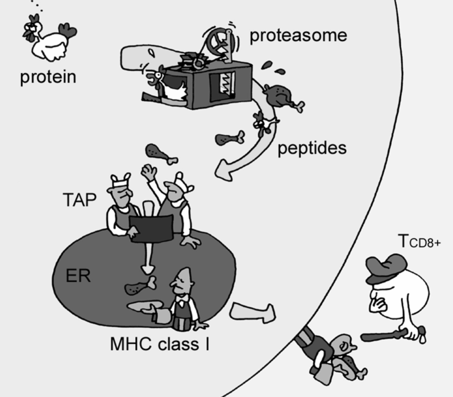
In this demo, we will be predicting if a given 9-mer peptide will be a 'strong-binder' SB, 'weak-binder' WB or a 'non-binder' NB to the MHCI variant HLA-A*02:01. We will be using a data set created by submitting 1,000,000 random 9-mers to netMHCpan-4.0 and predicting binding affinty to HLA-A*02:01. Based on the continuous binding affinty, each peptide is labeled SB, WB or NB. As n(SB) < n(WB) << n(NB), the data set was balanced by down-sampling, such that n(SB) = n(WB) = n(NB) = 7920. Thusly, the data set has a total of n(all) = 23760 data points. The data set was furthermore split into a train and test set, by random sampling 10% of the peptides. The data set is available here. It should be noted that this data set is derived from a model, so our final model in this example, will be a model of a model.
Click to expand
We need a few things installed before we're good to go, but I promise it'll be quick and painless!
You only need to do the following once!
Go ahead and head on over to The R Project for Statistical Computing and install the newest version of R. Then pop over to RStudio and get their brilliant IDE.
In order to use Keras and TensorFlow, we need to install them along with the TidyVerse framework. We also need PepTools for working with peptide data and lastly the ggseqlogo package for generating sequence logos. Fortunately, this is all straight forward using the ever brilliant Hadley Wickham's devtools:
install.packages("devtools")Now we load the devtools library, which will enable us to install the remaining requirements:
library("devtools")and then install requirements
install.packages("tidyverse")
devtools::install_github("rstudio/keras")
devtools::install_github("omarwagih/ggseqlogo")
devtools::install_github("leonjessen/PepTools")
Now simply run:
library("keras")Followed by
install_keras()That's it! Now we have all we need to be Data Science masters of the machine learning universe!
Here is a basic example of a deep FFWD ANN workflow (This example is adapted from this RStudio Keras tutorial).
First we clear the workspace to avoid unintentional reuse of old variables
rm(list=ls())Then we load the needed libraries
library("keras")
library("tidyverse")
library("ggseqlogo")
library("PepTools")
Then we load the example data
pep_file = "https://raw.githubusercontent.com/leonjessen/keras_tensorflow_demo/master/data/ran_peps_netMHCpan40_predicted_A0201_reduced_cleaned_balanced.tsv"
pep_dat = read_tsv(file = pep_file)The example peptide data looks like this
pep_dat## # A tibble: 23,760 x 4
## peptide label_chr label_num data_type
## <chr> <chr> <int> <chr>
## 1 LLTDAQRIV WB 1 train
## 2 LMAFYLYEV SB 2 train
## 3 VMSPITLPT WB 1 test
## 4 SLHLTNCFV WB 1 train
## 5 RQFTCMIAV WB 1 train
## 6 HQRLAPTMP NB 0 train
## 7 FMNGHTHIA SB 2 train
## 8 KINPYFSGA WB 1 train
## 9 WLLIFHHCP NB 0 train
## 10 NIWLAIIEL WB 1 train
## # ... with 23,750 more rows
Where peptide is a set of 9-mer peptides, label_chr defines whether the peptide was predicted by netMHCpan-4.0 to be a strong-binder SB, weak-binder WB or NB non-binder to HLA-A*02:01. label_num is equivalent to label_chr, only the predicted binding is coded into three numeric classes. Finally data_type defines whether the particular data point is part of the training set or the ~10% data left out and used for final evaluation. The data has been balanced, which we can see using TidyVerse methods to summarise the input data:
pep_dat %>% group_by(label_chr, data_type) %>% summarise(n = n())## # A tibble: 6 x 3
## # Groups: label_chr [?]
## label_chr data_type n
## <chr> <chr> <int>
## 1 NB test 782
## 2 NB train 7138
## 3 SB test 802
## 4 SB train 7118
## 5 WB test 792
## 6 WB train 7128
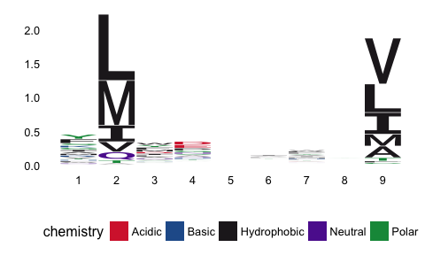
We can use the very nice ggseqlogo package to visualise the sequence motif for the strong binders:
pep_dat %>% filter(label_chr=='SB') %>% pull(peptide) %>%
  pssm_freqs %>% pssm_bits %>% t %>% ggseqlogo(method="custom")
From the sequence logo, it is evident that positions 2 and 9 in the peptide are of paramount importance for the MHCI-peptide binding. In fact these positions are known as the anchor positions.
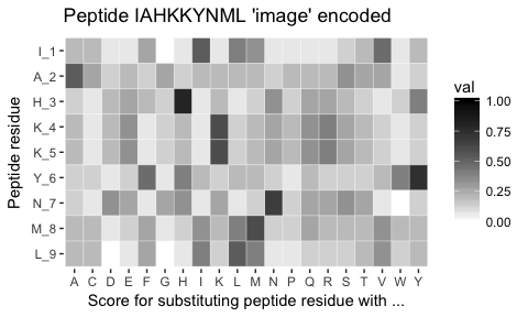
Each peptide is encoded using the BLOSUM62 matrix, such that each peptide becomes an 'image' matrix with 9 rows and 20 columns - Think of it as a QR code. We can visualise a peptide 'image' using pep_plot_images():
pep_ran(n = 1, k = 9) %>% pep_plot_imagesEach of these 'QR codes' define whether a given peptide is a strong-binder, weak-binder or non-binder. It is now our task to identify the pattern in the 'image' define which of the 3 classes the peptide belong to.
We are creating a model f, where x is the peptide and y is one of three classes SB, WB and NB, such that y ~ f(x). We need to define the x_train, y_train, x_test and y_test:
x_train = pep_dat %>% filter(data_type == 'train') %>% pull(peptide)   %>% pep_encode
y_train = pep_dat %>% filter(data_type == 'train') %>% pull(label_num) %>% array
x_test  = pep_dat %>% filter(data_type == 'test')  %>% pull(peptide)   %>% pep_encode
y_test  = pep_dat %>% filter(data_type == 'test')  %>% pull(label_num) %>% array
The x data is a 3-d array (a tensor) with n_rows x n_columns x n_slices = n_peptides x l_peptide x l_enc = 21384 x 9 x 20, i.e. all the 'images'/'QR codes' we generated. To prepare the data for training we convert the tensor into a matrix by reshaping width and height into a single dimension (9 x 20 peptide ‘images’ are flattened into vectors of lengths 180 and stacked as rows)
x_train = array_reshape(x_train, c(nrow(x_train), 180))
dim(x_train)
## [1] 21384 180
x_test  = array_reshape(x_test,  c(nrow(x_test), 180))
dim(x_test)
## [1] 2376 180
The y data is an integer vector with values ranging from 0 to 2. To prepare this data for training we encode the vectors into binary class matrices using the Keras to_categorical function:
y_train = to_categorical(y_train, y_train %>% table %>% length)
dim(y_train)
## [1] 21384 3
y_train %>% head(3)## [,1] [,2] [,3]
## [1,] 0 1 0
## [2,] 0 0 1
## [3,] 0 1 0
y_test  = to_categorical(y_test,  y_test  %>% table %>% length)
dim(y_test)
## [1] 2376 3
y_test %>% head(3)## [,1] [,2] [,3]
## [1,] 0 1 0
## [2,] 0 1 0
## [3,] 0 1 0
Now that we have the data, we can proceed to creating our TensorFlow model.
The core data structure of Keras is a model, a way to organize layers. The simplest type of model is the Sequential model, a linear stack of layers. We begin by creating a sequential model and then adding layers:
model = keras_model_sequential()
model %>%
  layer_dense(units  = 180, activation = 'relu', input_shape = 180) %>%
  layer_dropout(rate = 0.4) %>%
  layer_dense(units  = 90, activation  = 'relu') %>%
  layer_dropout(rate = 0.3) %>%
  layer_dense(units  = 3, activation   = 'softmax')
The input_shape argument to the first layer specifies the shape of the input data (a length 180 numeric vector representing a peptide 'image'). The final layer outputs a length 3 numeric vector (probabilities for each class SB, WB and NB) using a softmax activation function.
We can use the summary() function to print the details of the model:
summary(model)## ___________________________________________________________________________
## Layer (type) Output Shape Param #
## ===========================================================================
## dense_1 (Dense) (None, 180) 32580
## ___________________________________________________________________________
## dropout_1 (Dropout) (None, 180) 0
## ___________________________________________________________________________
## dense_2 (Dense) (None, 90) 16290
## ___________________________________________________________________________
## dropout_2 (Dropout) (None, 90) 0
## ___________________________________________________________________________
## dense_3 (Dense) (None, 3) 273
## ===========================================================================
## Total params: 49,143
## Trainable params: 49,143
## Non-trainable params: 0
## ___________________________________________________________________________
Next, compile the model with appropriate loss function, optimizer, and metrics:
model %>% compile(
  loss      = 'categorical_crossentropy',
  optimizer = optimizer_rmsprop(),
  metrics   = c('accuracy')
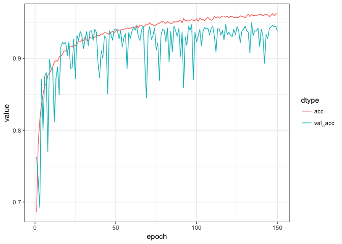
)We use the fit() function to train the model for 150 epochs using batches of 50 peptide ‘images’:
history = model %>% fit(
  x_train, y_train,
epochs = 150, batch_size = 50, validation_split = 0.2)We can visualise the training progress in each epoch using ggplot:
plot_dat = tibble(epoch = rep(1:history$params$epochs,2),
                  value = c(history$metrics$acc,history$metrics$val_acc),
                  dtype = c(rep('acc',history$params$epochs),
                            rep('val_acc',history$params$epochs)) %>% factor)
plot_dat %>%
  ggplot(aes(x = epoch, y = value, colour = dtype)) +
  geom_line() +
theme_bw()Finally we can evaluate the model’s performance on the original ~10% left out test data:
perf = model %>% evaluate(x_test, y_test)
perf
## $loss
## [1] 0.1823313
##
## $acc
## [1] 0.9372896
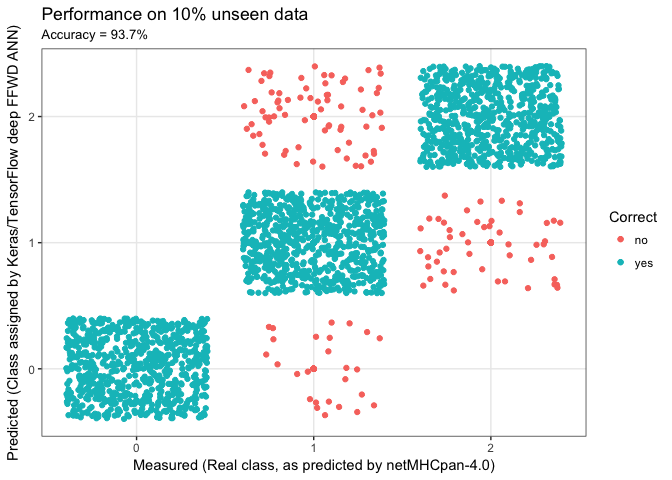
and we can visualise the predictions:
acc     = perf$acc %>% round(3) * 100
y_pred  = model %>% predict_classes(x_test)
y_real  = y_test %>% apply(1,function(x){ return( which(x==1) - 1) })
results = tibble(y_real = y_real, y_pred = y_pred,
                 Correct = ifelse(y_real == y_pred,"yes","no") %>% factor)
results %>%
  ggplot(aes(x = y_pred, y = y_real, colour = Correct)) +
  geom_point() +
  xlab("Measured (Real class, as predicted by netMHCpan-4.0)") +
  ylab("Predicted (Class assigned by Keras/TensorFlow deep FFWD ANN)") +
  ggtitle(label    = "Performance on 10% unseen data",
          subtitle = paste0("Accuracy = ", acc,"%")) +
  scale_x_continuous(breaks = c(0,1,2), minor_breaks = NULL) +
  scale_y_continuous(breaks = c(0,1,2), minor_breaks = NULL) +
  geom_jitter() +
  theme_bw()
That the end of this small demo - I hope you had fun!
Leon Eyrich Jessen
