learning-freak/Claims_Reserving

Claims Reserving in R

0. Contents

1. Introduction
2. Objective
3. Data Overview
4. Modeling
5. Conclusion
6. Bibliography

1. Introduction

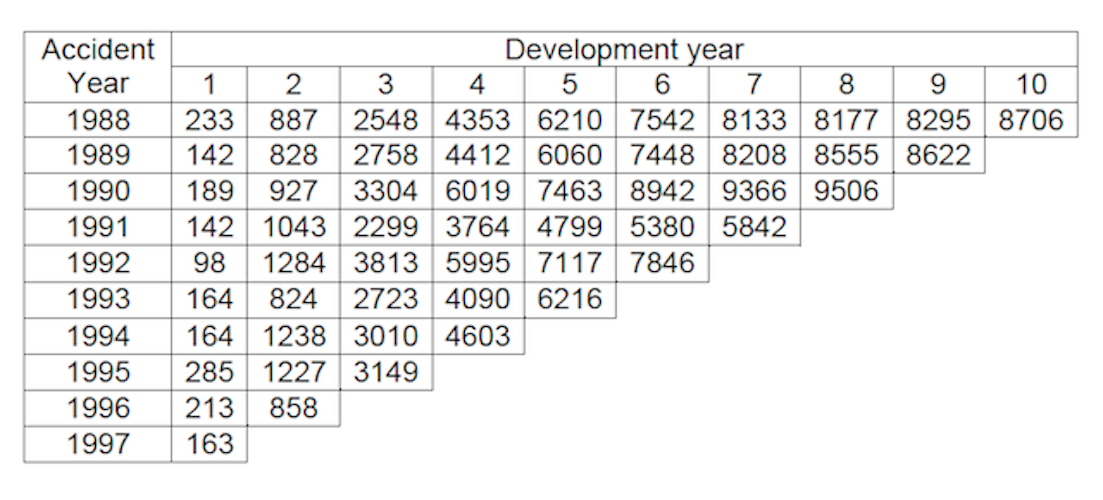
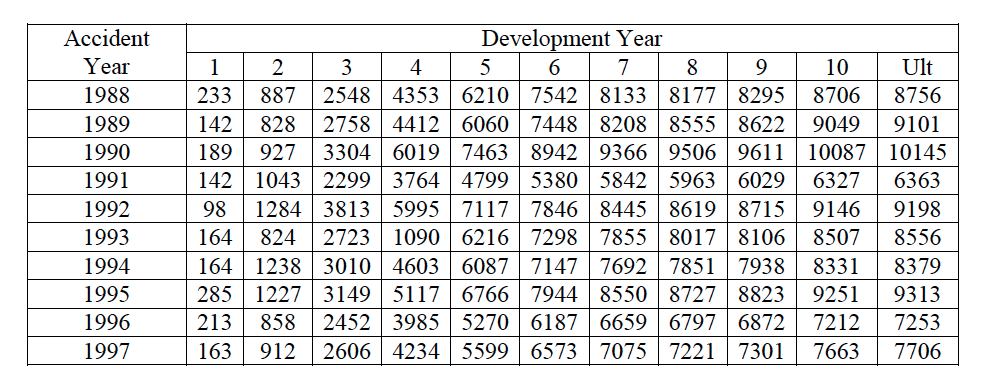
Glenn Meyers and Peng Shi provide databases that include major personal and commercial lines of business from U.S. property casualty insurers. For the purpose of this project, only the data involving Mercury Insurance Group will be used. The Claim Paid Losses in Other Liability Insurance for accident years in 1988-1997 form a development triangle as below. Presenting the data in a triangle structure is because (1) It shows the development of claims over time for each origin period; (2) “ChainLadder” package in R expect triangles as input data sets with development periods along the columns and the origin period in rows

2. Objective

I aim to forecast the future claims development for the bottom right half of the triangle. In other words, I am estimating unobserved values and quantify the outstanding loss liabilities for each origin year.

For the first part of this paper, I will be using the loss development factor deterministic method and applying the implemented Mack and Boot Strap Chain Ladder Stochastic Reserving models in R. I then approach the same problem with statistical approaches, building a log linear model and a log-linked GLM Poisson model. In conclusion, I summarize and discuss my achieved results for all the applied methods.

3. Data Overview

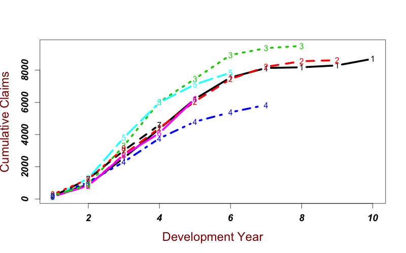
The cumulative claims development is visualized in the below Figure. Most of the insured incidents take 3-6 years to settle down and close. The growth rate is the highest after 2 - 3 years from the claims origin point but it does slow down with the increasing development period.

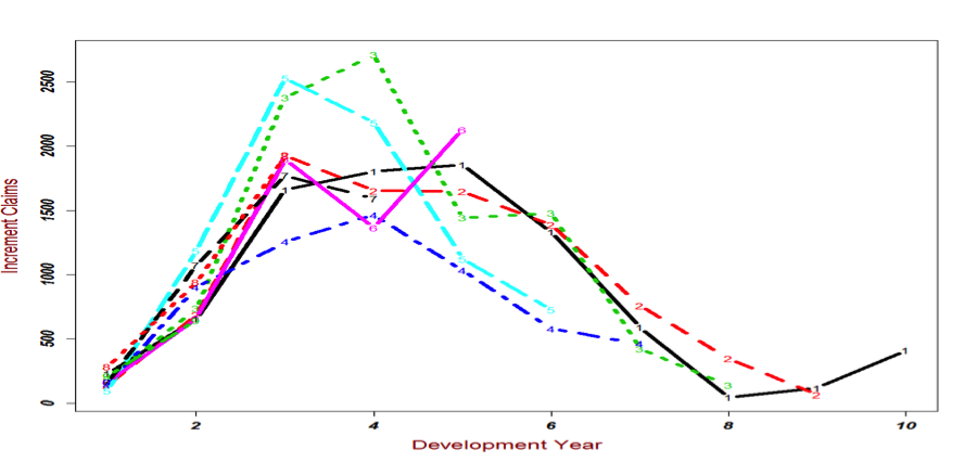
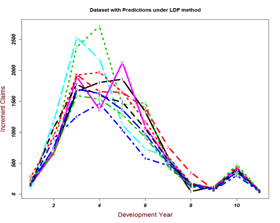
Incremental claims for the development years are displayed in the figure below. For this data set, the highest incremental claims come from the third, fourth and fifth development years. In general, the decreasing trend in claims development is visible.

##4. Modeling

4.1 Chain Ladder -- Reserving Methods

Chain Ladder methods use algorithms to forecast outstanding claims on the basis of historical data. They assume the cumulative claims losses for each business year develop similarly by delay year. Deterministic reserving method, Loss Development Factor method, uses the most basic chain ladder function. The Chain Ladder package in R has implementations of stochastic reserving models such as Mack, Munich, and Boot Strap Chain Ladder.

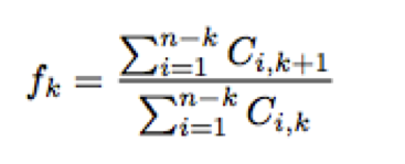
4.1.1 Loss Development Factor method -- Deterministic Reserving

Loss Development Factor method uses the basic chain ladder function, which link ratios are calculated as the volume weighted average development ratios of a cumulative loss development triangle from one development period to the next.

Since the oldest origin year is not fully developed, I extrapolate anther 100 development periods assuming a log-linear model. The link ratios then allow me to plot the expected claims development patterns.

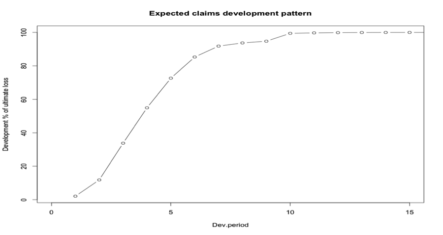
The link ratios are then applied to the latest known cumulative claims amount to forecast the next development period. An ultimate column is appended to the right to accommodate the expected development beyond the oldest year (10) of the triangle due to the tail factor (1.005696) being greater than unity.

Based on the estimated unobserved values, I can then draw the complete graph of Incremental claims for each origin year. The total estimated outstanding loss under this method is about 28778.

4.1.2 Mack chain ladder Implement – Stochastic Reserving

The Mack Chain Ladder model forecasts IBNR (Incurred But Not Reported) claims based on a historical cumulative claim triangle and calculates the standard error for the reserves estimates. It can be regarded as a weighted linear regression through the origin for each development period:

  lm(y ~ x + 0, weights=w/x^(2- alpha))

The Mack's method is implemented in the ChainLadder package via the function MackChainLadder. But this method will only works if accident years are independent. To ensure Mack’s Method is applicable for the dataset, we can check whether there are trends in the residual plots below.

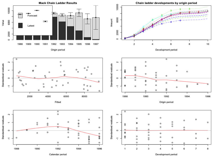
These residuals plot show the standardized residuals against fitted value, origin period, calendar period, and development period. The bottom left plot looks perhaps more like a level drop in calendar year immediately after 1992. However, the fit to the most recent years of data isn’t bad, so it might not be too problematic to use that forecast for the next year. I then access the loss development factors and the full triangle. Notice, not only that that the total amount of reserves is the same as using the deterministic method, but also the predict triangle.

4.1.3 Boot Strap Chain Ladder Implement– Stochastic Reserving

Boot Chain Ladder uses a two-stage approach. 1.Calculate the scaled Pearson residuals and bootstrap R times to forecast future incremental claims payments via the standard chain-ladder method. 2.Simulate the process error with the bootstrap value as the mean and using an assumed process distribution.

This two-stage boot strap approach is implemented in the Boot Chain Ladder function as part of the Chain Ladder package. As input parameters we provide the cumulative triangle, the number of bootstraps and the process distribution to be assumed: BootCL=BootChainLadder(top_tri,R=800,process.distr="od.pois")

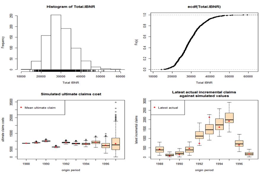
Top left: .Histogram of simulated total IBNR
Top right: Empirical distribution of total IBNR
Bottom Left: Box-whisker plot of simulated ultimate claims cost by origin period
Bottom right: Box-whisker plot of simulated ultimate claims cost by origin period

The set of reserves obtained in this way forms the predicted distribution, from which summary statistics such as mean, prediction error and quantiles can be derived. The distribution of the IBNR appears to follow a log-normal distribution, so let’s keep that in mind.

4.2. Statistical Modeling

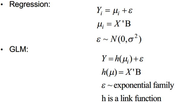
There are three main categories in statistical predictive modeling: Classical Linear Models, Generalized Linear Models(GLMs), and Data Mining. An easy way to think about GLMs is as models that generalize the error term distribution to a family of distributions, called exponential family. It includes normal, binomial, Poisson, and gamma distributions among others. In addition, the response variable in GLM is related to linear regression through a link function. Common used link functions are Identity, Inverse, Inverse Squared, Log and Logit. The differences between Linear Models and GLMs is as followed.

4.2.1 Pre-Analysis

The chain ladder methods uses cumulative claims, but statistical approaches uses the incremental claims. The R package ChainLadder comes with two helper functions, cum2incr and incr2cum. They can transform cumulative triangles into incremental triangles and vice versa. The development of the incremental claims is shown in below figure individually for each origin period. we can see that the outcome is a continuous outcome, but is right skewed and always positive.

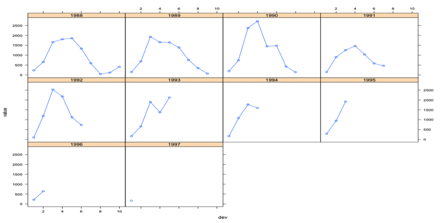
4.2.2 Linear Model with log-transformed outcome

Since the distribution has a positive skew, taking a natural logarithm of the variable helps fitting variable into a model. Thus, that is the first model I build, and carry out the linear regression with

  lm(log(inc_loss) ~ as.factor(dev) + as.factor(ay), data=inc_data)

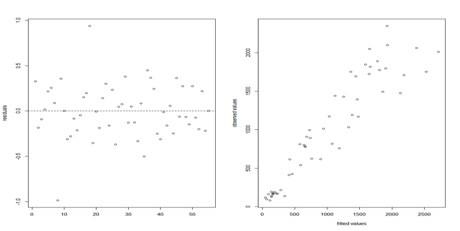
Despising a few outliers, the residual plot below look quite well behaved. In an ideal case, the observed values vs. the fitted values plot should also be distributed along the diagonal. The total correlation coefficient between the fitted and observed value is 0.8827, thus I decided to investigate further.

4.2.3 Log-linked GLM Poisson

Since the outcome is right skewed and always positive, the incremental losses seem to be Poisson distributed. Thus I choose using the Poisson family in GLM. The link function is log() to be consistent with the previous linear model, thus the model is modeling the following:

  glm(inc_loss ~ factor(ay) + factor(dev), data=inc_data, family=poisson("log"))

Looking at the residual plot below, we can see that I was able to successfully get rid of the residual outlines from the previous model. In fact, the residuals is stationary with zero mean, and constant variance.

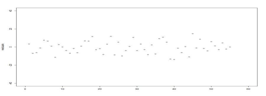
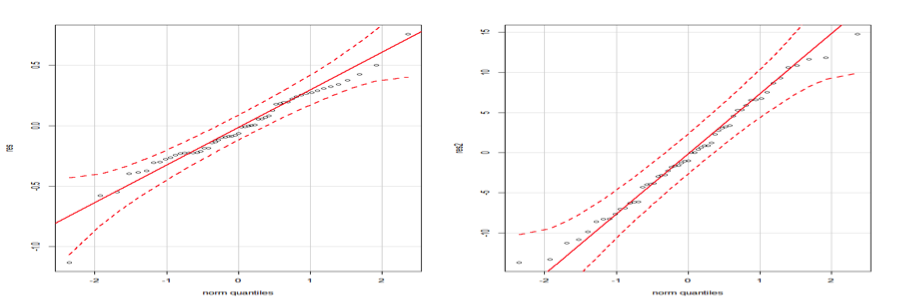
The observed values vs. the fitted values plot is distributed along the diagonal. The relationship between observed and fitted value is satisfying, the correlation coefficient is 0.9497. For model fit checking purpose, I also compare the qqPlot(s) from these two models. And the log-linked GLM Poisson indeed fits the data better.

4.2.4 Prediction of the claims

The intercept term estimates the first log-payment of the first origin period. The other coefficients are then additive to the intercept. Thus, the predictor for the second payment of 1989 would be exp(5.22139 + 0.03866 + 1.52445)=884.038. The second column in the output above gives us immediate access to the standard errors. Based on those estimated coefficients, we can predict the incremental claims payments. The total amount of reserves is the sum of incremental predicted payments beyond year 1997.

   sum(predict(gl,type="response", newdata=subset(Claims, cal > 1997)))

For a better illustration of how fitted my model capture the observed claims development. The following graph is provided. The red lines represent the observed incremental losses. The blue lines represent the model fitted values, the green lines stand for the predicted incremental losses.

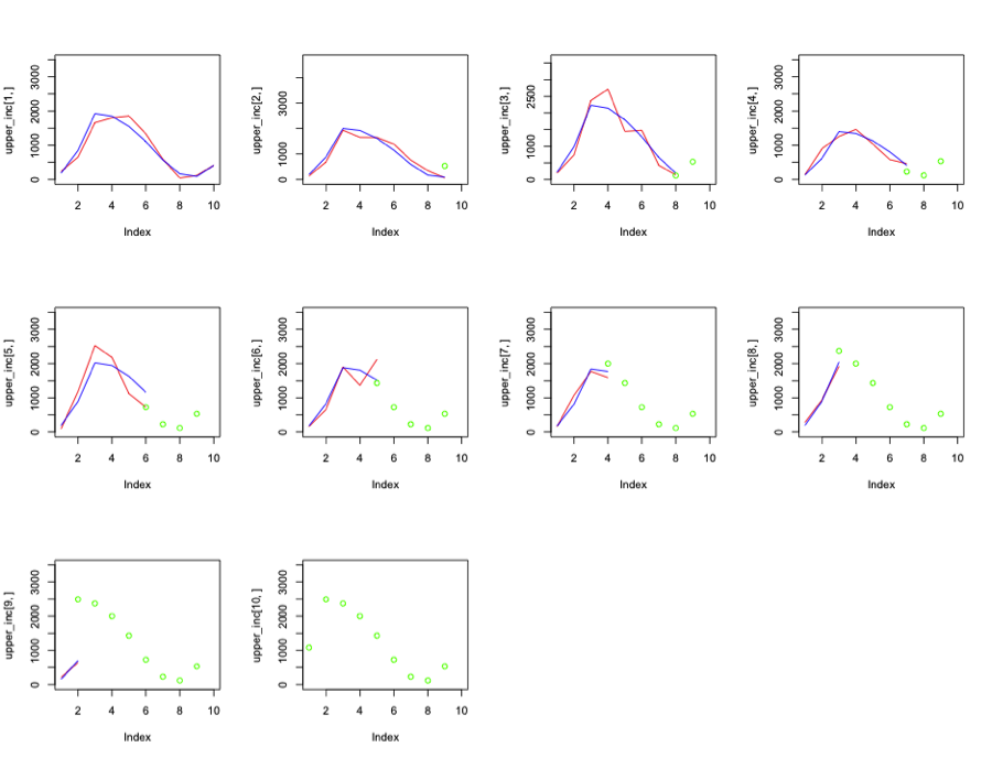
There are some overestimations and underestimations and underestimations at the middle year of the claim development. But the fit is satisfying. The total amount of financial instruments that need to be held in claims reserve under this model is 28779.

5. Conclusion

The main goal of this paper was to learn the preliminary reserving techniques for insurance companies like Merry Insurance Group. Once an appropriate model is built, the predicted claim reserve is approximately around 28778, whether I was using the deterministic method, applying the implemented stochastic reserving models, or building statistical models.