Density Estimation Forests in Python

Kernel Density Estimation in Random Forests

Usage

Running --help

usage: density_forest.py [-h] [-l LEAF] [-d DATA] [-g GRANULARITY]

randomforest-density: density estimation using random forests.

optional arguments:
  -h, --help            show this help message and exit
  -l LEAF, --leaf LEAF  Choose what leaf estimator to use (Gaussian ['gauss']
                        or KDE ['kde'])
  -d DATA, --data DATA  Path to data (.npy file, shape (sample_zie, 2)).
  -g GRANULARITY, --granularity GRANULARITY
                        Number of division for the Grid

Run demo (will produce all the plots seen below):

python3 density_forest.py -l kde

Run own data:

python3 density_forest.py -d data_test.npy -l gauss

Introduction

In probability and statistics, density estimation is the construction of an estimate, based on observed data, of an unobservable underlying probability density function. The unobservable density function is thought of as the density according to which a large population is distributed; the data are usually thought of as a random sample from that population.

Random forests are an ensemble learning method that operate by constructing a multitude of decision trees and combining their results for predictions. Random decision forests correct for decision trees' habit of overfitting to their training set.

In this project, a random forests method for density estimation is implemented in python. Following is the presentation of some of the steps, results, tests, and comparisons.

Random Forest Implementation

In this implementation, axis aligned split functions are used (called stumps) to build binary trees by optimizing the entropy gain at each node. The key parameters to select for this method are: tree depth/entropy gain threshold, forest size, and randomness.

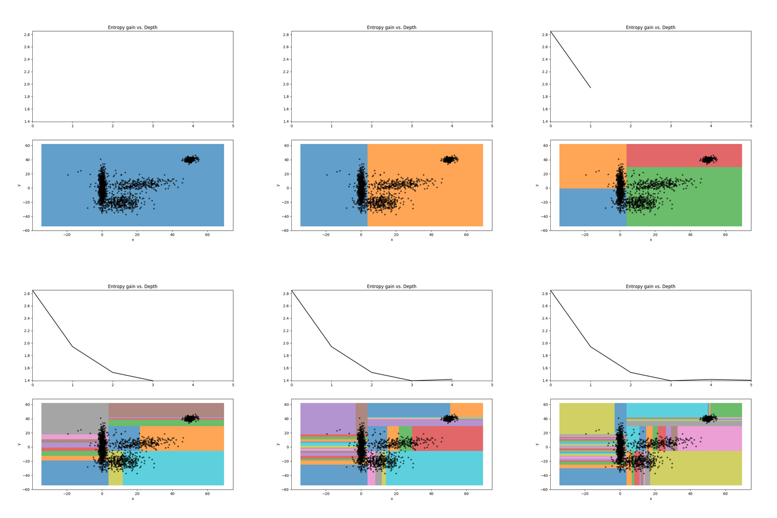
The optimal depth of a tree will be case dependent. For that reason we first train a small set of trees on a fixed depth (tune_entropy_threshold method, parameters n and depth). Unlike forest size, where an increase will never yield worse results, a lax stop condition will lead to overfitting. The entropy gain is strictly decreasing with depth, as can be seen in the animation below:

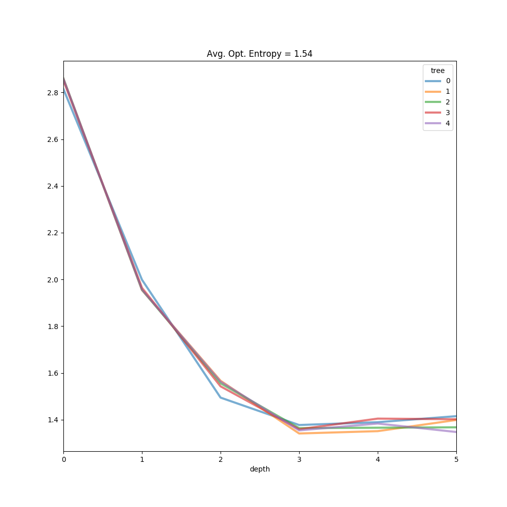
Optimizing the entropy gain threshold is an ill-posed regularization problem, that is handled in this implementation by finding the elbow point of 'maximum depth' (point furthest from the line connecting the the function's extremes), and averaging it out over n, as we can see here:

This step is expensive, since the depth is fixed with no a priori indication of where the optimal threshold is, and the number of leafs that need to be fitted grows exponentially. A better approach would be to implement an online L-curve method (such as the ones discussed here) as a first pass to avoid initial over-splitting (pending).

From Decision Forests for Classification, Regression, Density Estimation, Manifold Learning and Semi-Supervised Learning:

A key aspect of decision forests is the fact that its component trees are all randomly different from one another. This leads to de-correlation between the individual tree predictions and, in turn, to improved generalization. Forest randomness also helps achieve high robustness with respect to noisy data. Randomness is injected into the trees during the training phase. Two of the most popular ways of doing so are:

These two techniques are not mutually exclusive and could be used together.

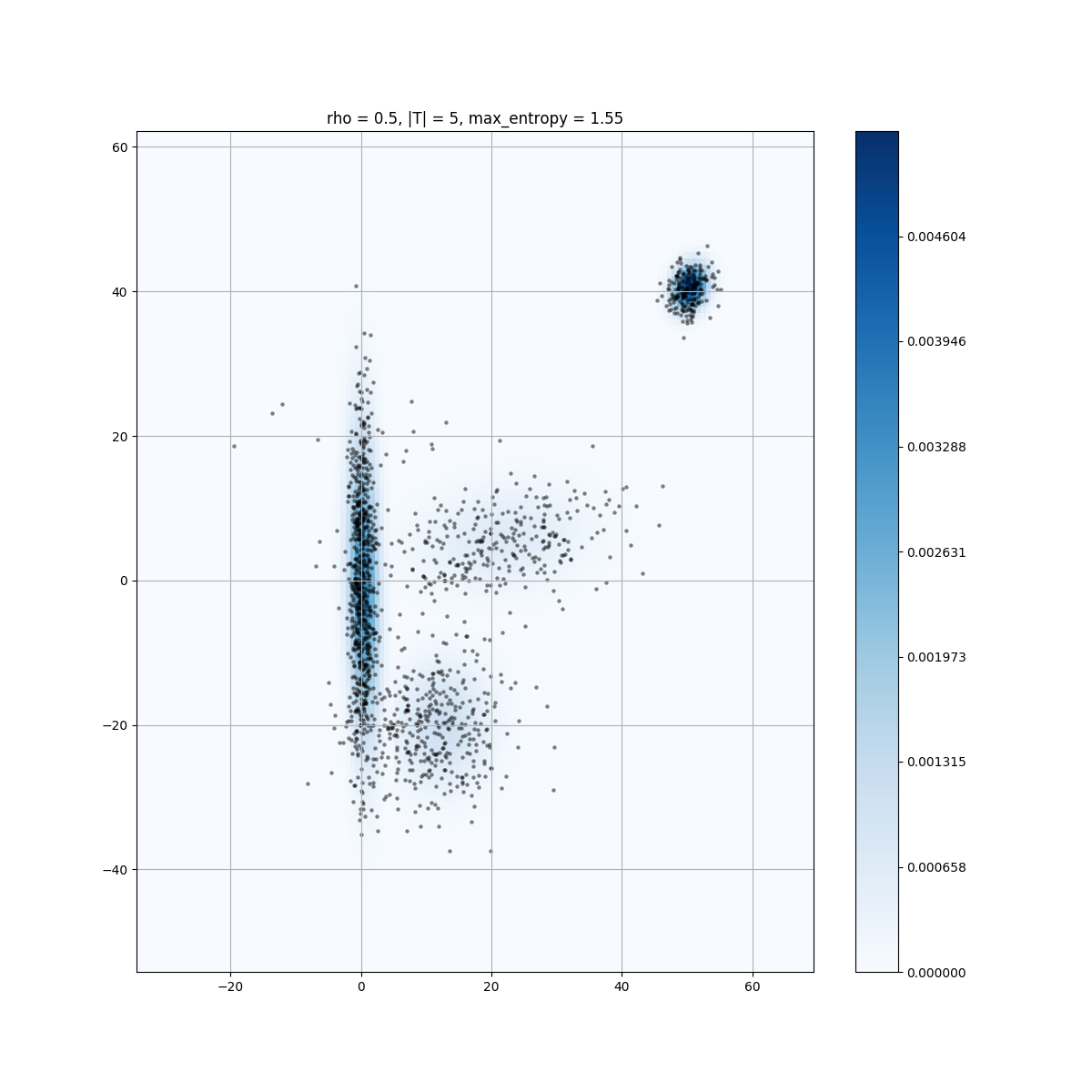
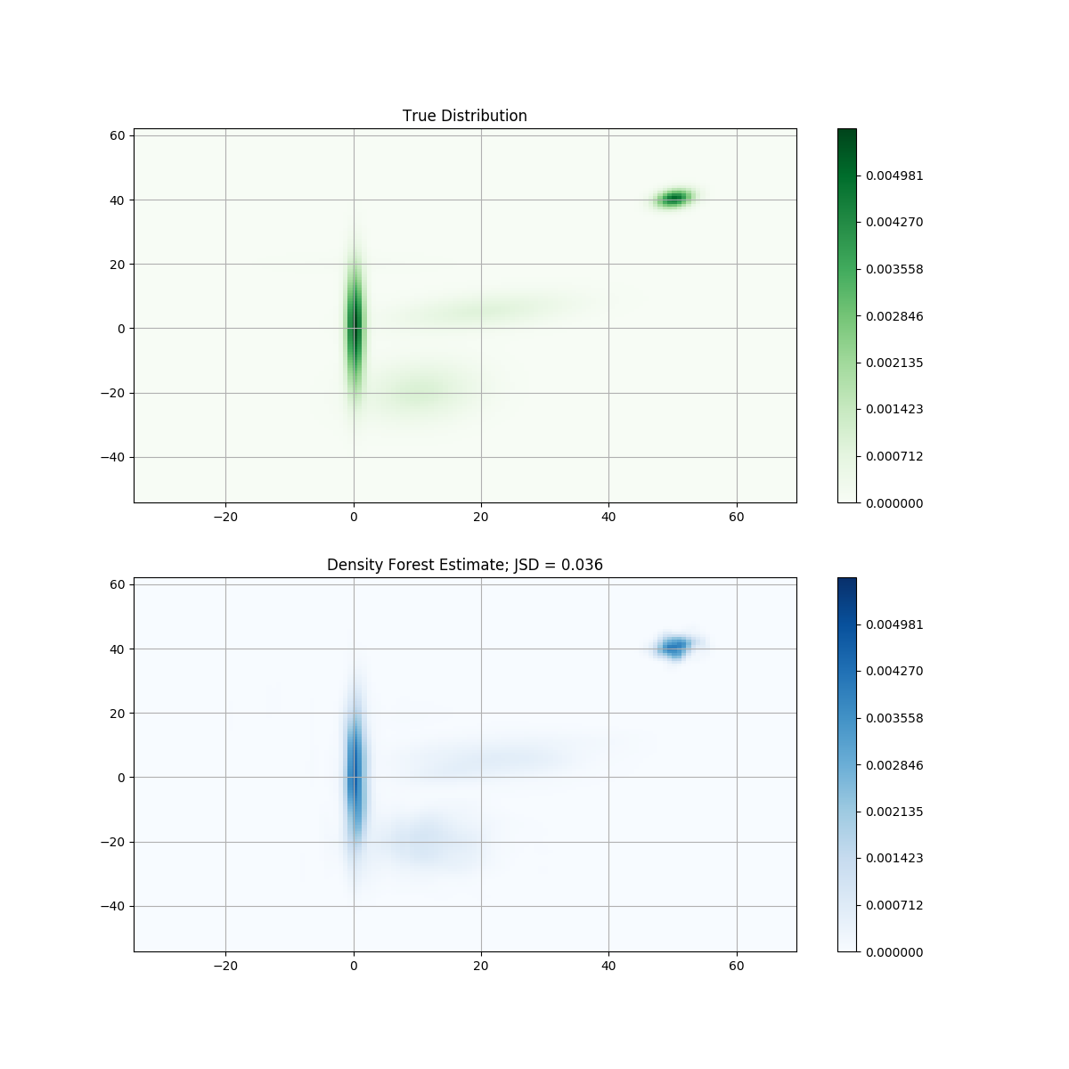
The method is tested by sampling a combination of gaussians. In order to introduce randomness the node optimization is randomized by parameter rho, with the available parameter search space at each node split proportional to it. With a 50% rho and 5 trees, we see the firsts results below:

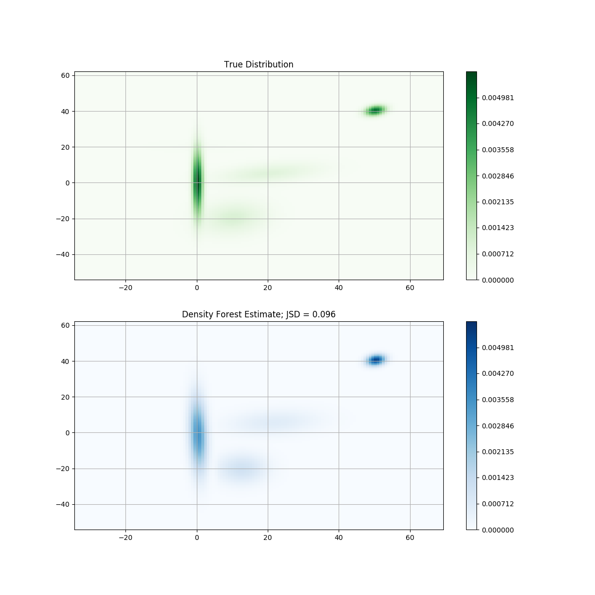
Performance is harder to measure when using random forests for density estimation (as opposed to regression or classification) since we're in the unsupervised space. Here, the Jensen-Shannon Divergence is used as a comparison measure (whenever test data from a known distribution is used).

Leaf prediction using KDE

One of the main problems of Kernel Density Estimation is the choice of bandwidth. Many of the approaches to find it rely on assumptions of the underlying distribution, and perform poorly on clustered, real-world data (although there are methods that incroporate an adaptive bandwidth effectively).

The module can work with any imlementation of the Node class. In these first examples the NodeGauss class is used, by fitting a gaussian distribution at each leaf. Below can be seen the results of using NodeKDE, where the compactness measure is still based on the gaussian differential entropy, but the leaf prediction is the result of the KDE method. By looking for splits that optimize fitting a gaussian function, many of the multivariate bandwidth problems that KDE has are avoided, and Silverman's rule for bandwidth selection can be used with good results:

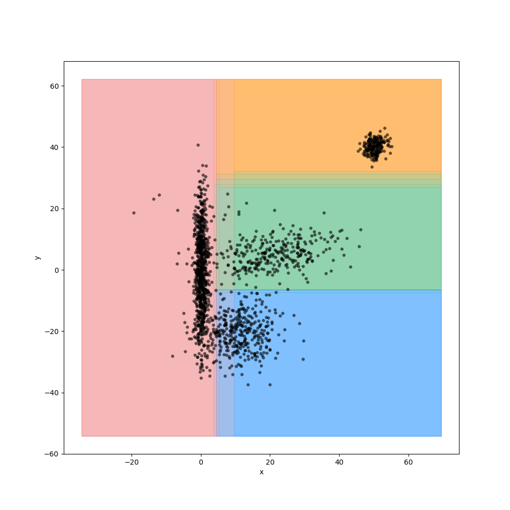
Although it produces an overall much better JSD, it's worth noting that the top right 'bump' is overfitting the noise more. This is expected since the underlying distribution of our test data is a combination of Gaussians, and if a leaf totally encompasses a bump (as can be seen in the forest representation below), then fitting a Gaussian function will perform better than any non parametric technique.

To do

Try other entropy gain functions / compactness measures.
Use online L-curve method for entropy threshold optimization.
Other bottlenecks.
Refactor to reuse framework in classification and regression.
Fit unknown distributions / performance.
Use EMD as comparison metric.

ksanjeevan / randomforest-density-python