The example is an educational version of a Higgs to two tau lepton analysis based on NanoAOD-like samples from the CERN Open Data portal. To fit the computational effort of the analysis in the scope of the workshop, the samples are reduced beforehand. See the documentation below for the single steps.
Features:
- The analysis has the common steps of skimming, histogramming and plotting/fitting
- The skimming and histogramming workflow is parallelized on file basis and all results are just merged for the plotting or fitting.
- No experiment specific software needed, no experiment policies attached to the data or code.
- Minimal software dependencies (ROOT and Python), running on all major CERN infrastructure (lxplus, SWAN, all CVMFS enabled machines)
- The analysis workflow is scripted in bash so we can transfer this during the workshop to any workflow management software such as ReANA.
- Supplementary webpage with documentation and exercises
- Indico agenda of the event
- Record on the CERN Open Data portal used as baseline
The analysis needs only ROOT (6.16 or later) and Python (2 and 3 should work).
TODO: People will go for the first option whatever it is, so let's shuffle accordingly.
You can run on any CVMFS enabled machine such as lxplus sourcing an LCG release (don't forget to select the correct platform if you don't use lxplus with CentOS 7). Run the following commands to connect to lxplus with your CERN account and source the correct software stack.
ssh your_user@lxplus.cern.ch
source /cvmfs/sft.cern.ch/lcg/views/LCG_95/x86_64-centos7-gcc8-opt/setup.shInstall conda and ROOT following the instructions here. Works for Linux and macOS.
cd /path/to/analysis/repodocker run -it --rm -v $PWD:/analysis -w /analysis rootproject/root:6.26.10-conda /bin/bashTo reduce the initial samples to a fraction of the size, call the bash script reduce.sh, which processes all relevant samples with a constant reduction factor.
The already reduced samples are placed on a public EOS space here: root://eospublic.cern.ch//eos/root-eos/HiggsTauTauReduced/
Details:
-
[Data] Locally on an SSD, 6.5GB, 10% of the original samples, represents data and simulation of about 1.1fb-1 of the data taken in 2012 with CMS
-
[System] Consumer laptop, single core, on reduced initial samples, everything fully sequentially
Runtime:
- [Skimming] 2m30s (local files as described above), 6m (streamed via XRootD)
- [Histograms] 40s
- [Plotting] Instant
- [Fit] Almost instant
Note that skimming and histogram production can be run seamlessly in multi-threading mode. I removed the feature for now so that we don't break any workflow later on (container, ReANA, ...) but we could improve the runtime by a factor of around N (N being the number of threads used / physical cores).
The first analysis step skims the NanoAOD-like samples with a baseline selection and finds valid muon-tau pairs. The output is written as a flat ntuple for further processing. Run bash skim.sh /path/to/dir/with/samples /path/to/output/dir to skim all (reduced) samples.
You have the option to download the samples beforehand or stream the data. To download the samples, run bash download.sh /path/to/output/dir and point for the skim.sh script to this directory. To stream the data, run bash skim.sh root://eospublic.cern.ch//eos/root-eos/HiggsTauTauReduced/ /path/to/output/dir.
Next, we make histograms of all variables and physics processes for later plotting. Call bash histograms.sh /path/to/dir/with/skims /path/to/output/dir to run the workflow.
Finally, we make the physics results by combining the histograms. Run bash plot.sh /path/to/histograms.root /path/to/output/dir for this step.
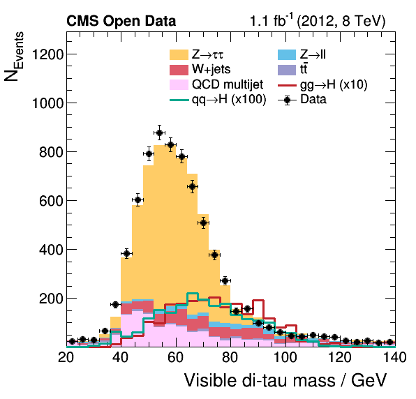
The resulting plots are added to this repository as reference, e.g., see here the visible mass of the di-tau system:
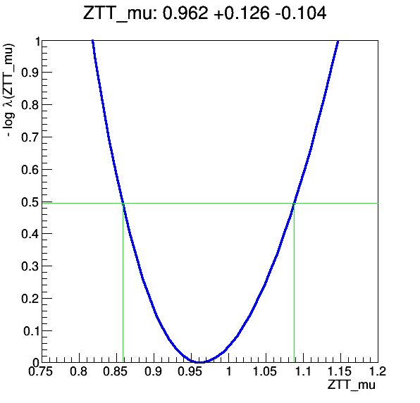
Optionally, we can fit the cross-section of any process using the histograms also used for plotting. In the implemented example, we use the HistFactory of ROOT to fit the signal strength of the Z to two tau lepton process. Call bash fit.sh /path/to/histograms.root /path/to/output/dir to produce the following profile:


