MicroCrop - Crop Solver by Adam

Motivation

This application was created to practice C++ & CUDA C/C++ coding after completing NVIDIA Fundamentals of Accelerated Computing with CUDA C/C++.

Since the beginning of my university studies of agricultural engineering, simulating agricultural equipment is my passion. I was especially interested in new technologies to simulate processing of agricultural materials. One day I ran into an interesting study on mass-spring systems: Oussama Jarrousse: Modified Mass-Spring System for Physically Based Deformation Modeling. The author used this method to simulate human organs like breast and heart, so I thought it can be used for agricultural materials too. Nonetheless, implementing this method into a C++ & CUDA C/C++ code seemed to be a perfect exercise to practice my new knowledge.

My certificate:

Short description

In the simulation, each component (body) is consisted of tetrahedral cells. The mechanical behaviour of the cells are defined by axial and rotational springs and dampers. Contact is detected among the cells that belong to the same or different components. The mechanical behaviour of the contact between two components is determined by the interaction properties such as contact stiffness and coefficient of static friction. The components are able to deform according to the contact and external forces acting on them. The cells can be damaged and this can result in breakage of the component. Initial and boundary conditions can be defined onto the components at the beginning of the simulation. Nonetheless, external forces (like gravity) and fixed velocities can be applied onto the components as well.

Input parameters:

Tetrahedral mesh for each component;
Material definition for each component;
Interaction definition among the components;
Initial conditions;
Boundary conditions;
External forces;
Fixed velocities;
Solver settings;
Save setting.

Result files:

Log file (TXT) with solver messages;
Node output file (VTK);
Cell output file (VTK);
Face output file (VTK);
Axial spring output file (VTK);
Rotational spring output file (VTK);
Contact output file (VTK);
External force output file (VTK).

The VTK output files can be processed and visualized in Paraview.

The solver was developed in Microsoft Visual Studio 2019 by using ISO C++14 standard and NVIDIA CUDA 11.3.

Small examples

In this section you can find small examples that show some of the capabilities of the solver.

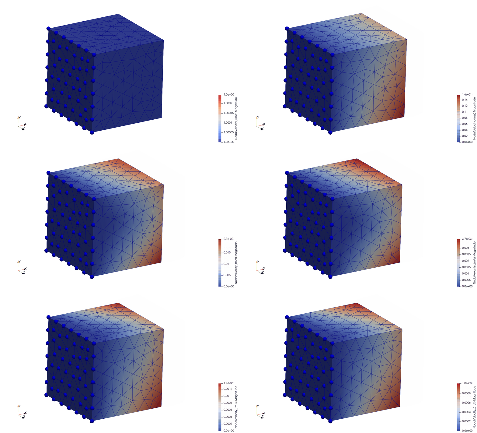
One-side fixed cube with initial velocity

In this example, a single cube (size: 0.01 x 0.01 x 0.01 m) is fixed on one side (all 3 DoFs) while initial velocity of 1.0 m s ^-1 in direction X and gravitational acceleration of -9.81 m s ^-2 in direction Y are applied on it. The simulation contains the following elements:

343 nodes;
4548 faces;
1137 cells;
3411 axial and
3411 rotational springs.

The material was isotropic, so all the three anisotropy axes had the same physical and mechanical properties. The cube is also homogeneous, so all the cells had the same material definiton. For the sake of a quick solve, I used a relatively high density (1200 kg m ^-3) and a very low axial spring stiffness (1.0 N m ^-1). The system was also overdamped by using a viscous damping of 1e-2 N s m ^-1. Overall, I believe it is a jelly-like material.

The total simulation time was 0.1 sec and it was solved with a time step of 1e-5 sec on 12 CPU threads. The total solving time was 66 seconds. For more details, you can find the input and output files here:

\0_INPUT\SingleCube_Fixed_InitialVelocity_Gravity
\1_OUTPUT\SingleCube_Fixed_InitialVelocity_Gravity

Below, you can see the visualization of the results in Paraview. The cells are visualized by magnitude nodal velocity. The boundary conditions (fixed nodes) are visualized by blue spheres on the left side of the cube.

Cube tensile test

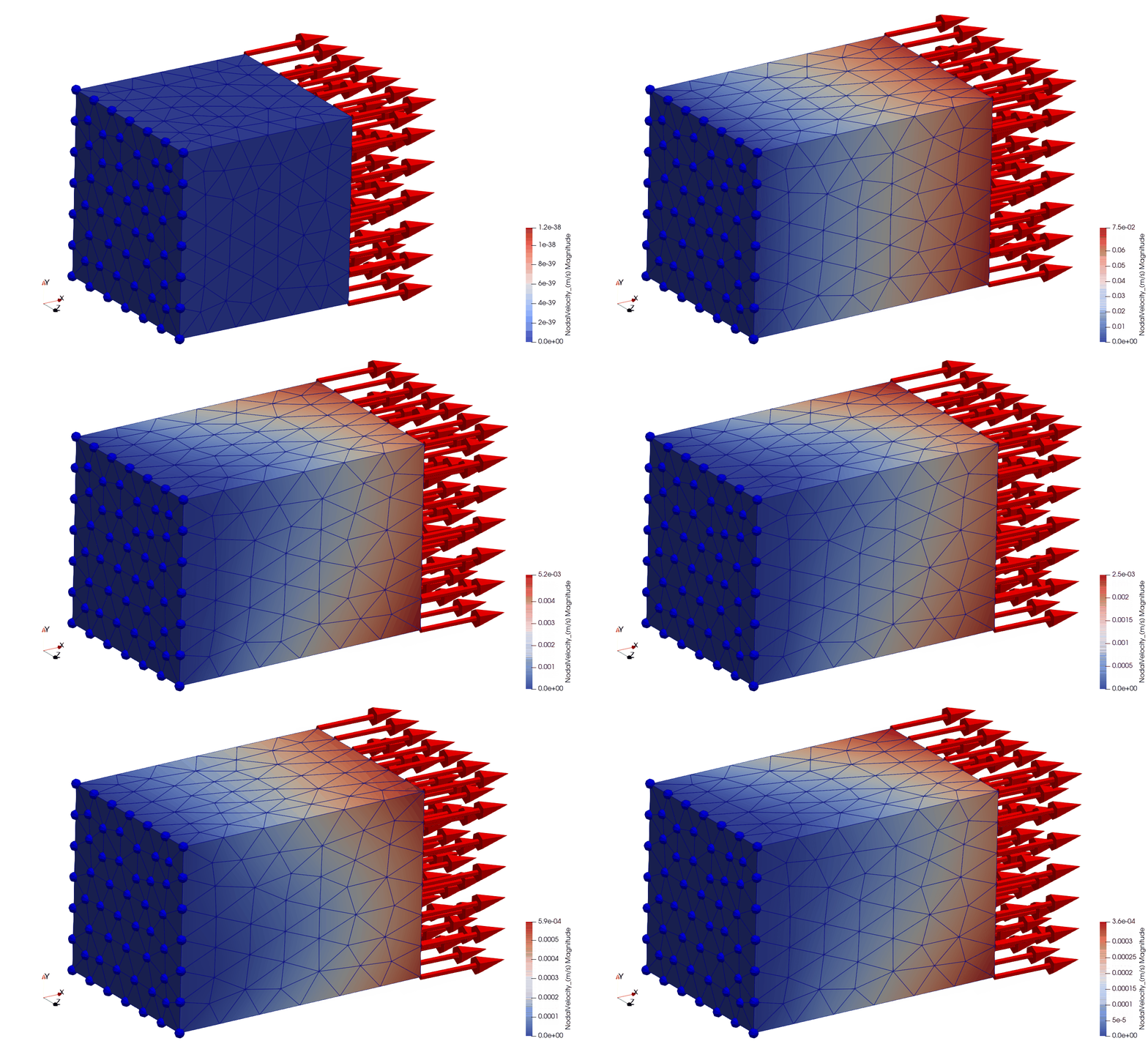
In this example, a single cube (size: 0.01 x 0.01 x 0.01 m) is fixed on one side (all 3 DoFs) while an external force of 1e-3 N in direction X is applied on each node on the other side of the cube. The simulation contains the following elements:

343 nodes;
4548 faces;
1137 cells;
3411 axial and
3411 rotational springs.

The total simulation time was 0.1 sec and it was solved with a time step of 1e-5 sec on 12 CPU threads. The total solving time was 64 seconds. For more details, you can find the input and output files here:

\0_INPUT\SingleCubeTensileTest
\1_OUTPUT\SingleCubeTensileTest

Sphere - cube eccentric collision

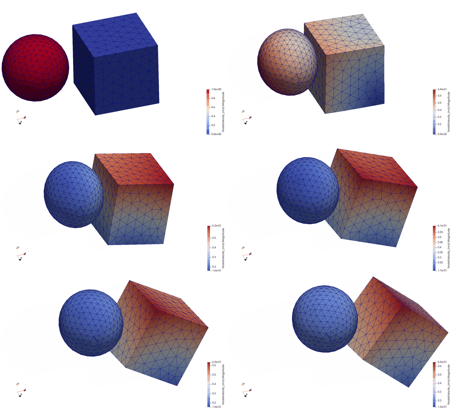
In this example, there are two components: a sphere and a cube. The sphere has a diameter of 0.01 m, while the size of the cube is 0.01 x 0.01 x 0.01 m. The center of the sphere is located above the center of the cube by 0.002 m, thus they are eccentric. The sphere has an initial velocity of 1.0 m s ^-1 in direction X. The cube is floating in the space without having any initial or boundary conditions.

The simulation contains the following elements:

977 nodes;
14864 faces;
3716 cells;
11148 axial and
11148 rotational springs.

For both components, the material was isotropic, so all the three anisotropy axes had the same physical and mechanical properties. The components are also homogeneous, so all the cells had the same material definiton. For the sake of a quick solve, I used a relatively high density (1200 kg m ^-3) and a very low axial spring stiffness (1.0 N m ^-1). The system was also overdamped by using a viscous damping of 1e-2 N s m ^-1. Overall, I believe it is a jelly-like material.

As to the interaction properties, the coefficient of static friction was set to be 0.2 between the two components. The normal contact stiffness was set to 2e3 N m ^-1, while the tangential contact stiffness was 1e3 N m ^-1.

The total simulation time was 2.5e-2 sec and it was solved with a time step of 1e-6 sec on 12 CPU threads. The total solving time was 367 seconds. For more details, you can find the input and output files here:

\0_INPUT\SphereCube_Collision
\1_OUTPUT\SphereCube_Collision

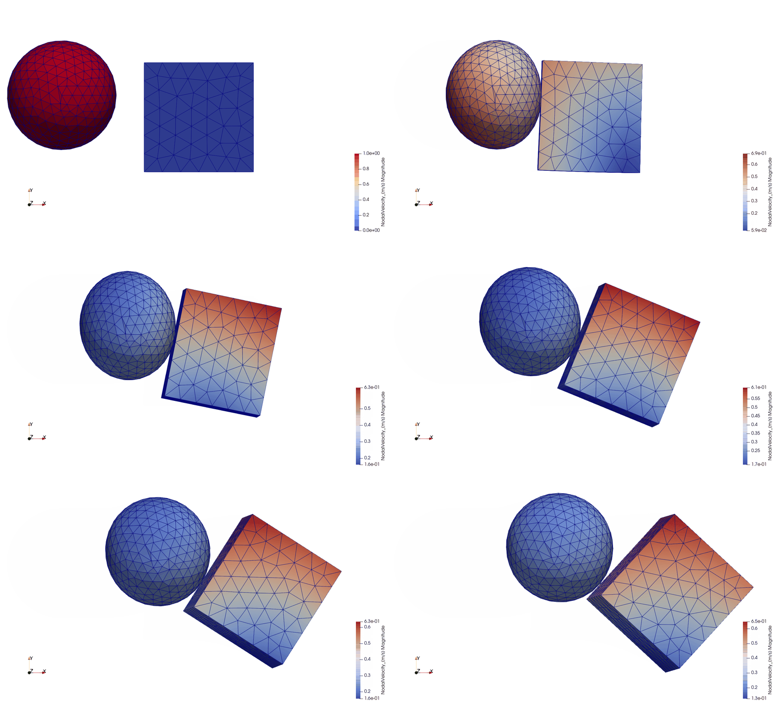
Below you can see the eccentric collision of the two components:

ISO view of the collision: components are visualized by magnitude nodal velocity;
Side view of the collision: components are visualized by magnitude nodal velocity;
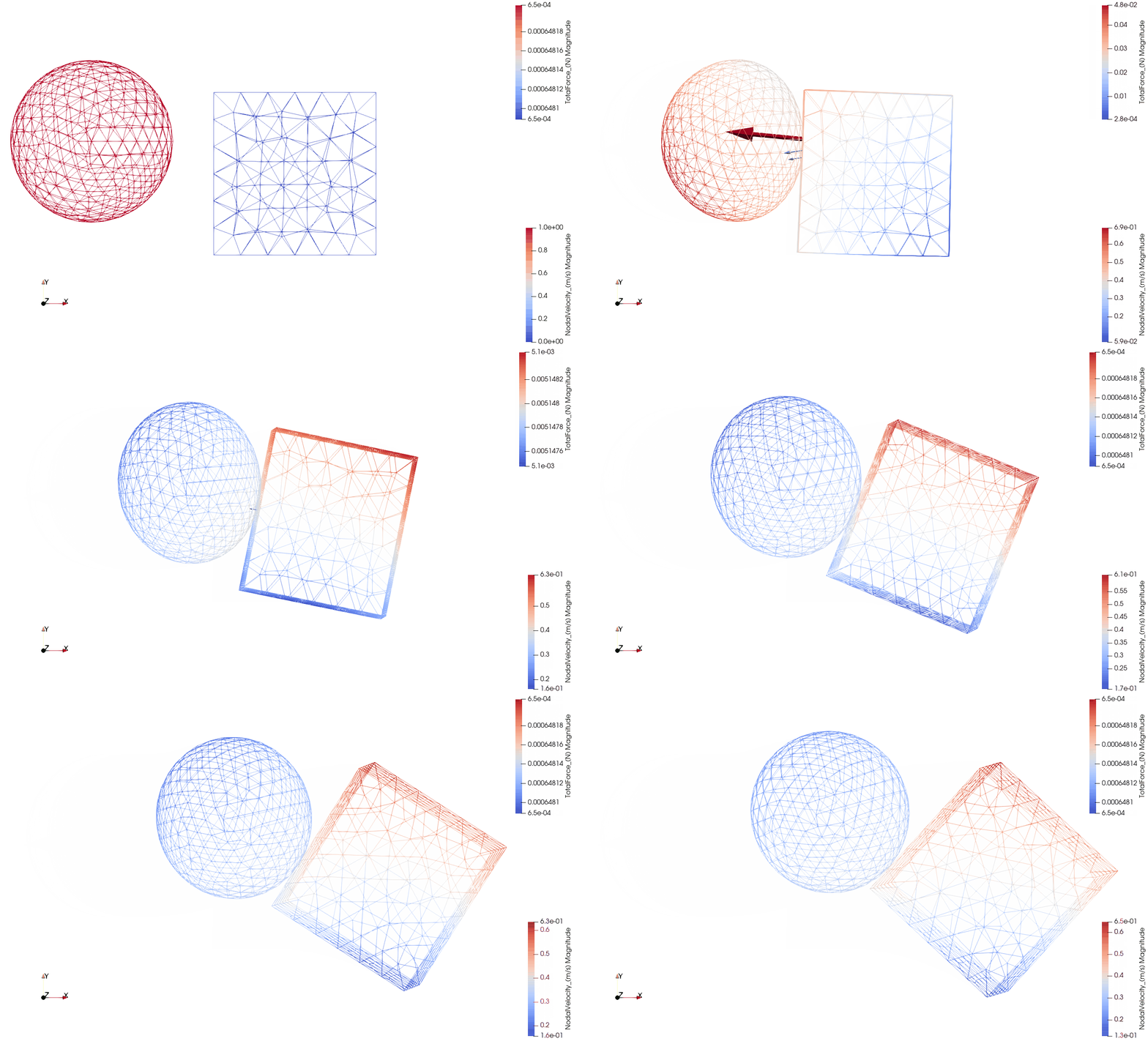
Wireframe view with the total contact forces being visualized by arrows.

ISO view:

Side view:

Wireframe with contact forces:

A real life application - Corn stalk simulation

The purpose of this exercise is to prove the following hypotheses:

The mass-spring simulation technique [1.] can be utilised on agricultural materials;
A calibrated mass-spring model is capable of predicting the physical and mechanical behaviour of agricultural materials.

For the test of interest, the transversal compression of a corn stalk section was selected, see below. The same physical and virtual tests were performed during my PhD research. For more details, you can find my dissertation [2.] in the documentation folder.

The presented corn stalk model was not completely calibrated. I used the same iterative method taht was developed during my PhD research [2.] for the Discrete Element Model (DEM) calibration. In the future, I would like to test other calibration approaches involving machine learning.

The simulation files are located here:

Geometry and mesh: \0_INPUT\CornStalk\Geometry_Mesh
Corn stalk material creator Python script: \0_INPUT\CornStalk\MaterialCreation_Python
Solver input files: \0_INPUT\CornStalk\SolverInput
Result files: \1_OUTPUT\CornStalk_FinalRun

Input parameters

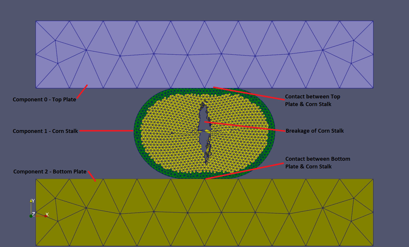
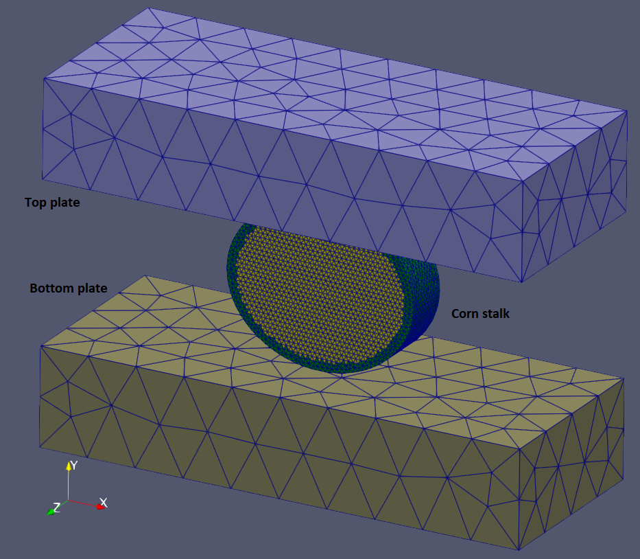
There are three components in the simulation: top plate, cron stalk and bottom plate, see below. All the geometries and meshes were created in Gmsh. Explaining the usage of Gmsh is not part of this documentation. You can find its official reference manual here.

The dimensions of the top and bottom plates are 0.05 x 0.01 x 0.02 m. The corn stalk has a perfect ellipse cross section with the size of the major and minor axes being 9.75e-3 and 8.2e-3 m, respectively. The length of the corn stalk section is 5e-3 m. These dimensions were defined based on my previous researach. [2.]

For the top and bottom plates a coarse, while for the corn stalk a relatively fine mesh was used. The top and bottom plates were meshed in the same way by setting the largest element size to be 1e-2 m. However, the defined largest element size for the corn stalk mesh was 5e-4 m.

The top plate has a fix velocity of -3.33 m s ^-1 in direction Y, while the bottom plate is fixed. The corn stalk section has no initial or boundary conditions. As an external force, gravitational field of -9.81 m s ^-2 was applied globally in direction Y.

Interaction properties were defined between the top plate & corn stalk, corn stalk & corn stalk and corn stalk & bottom plate. All the interaction properties were set to be the same. The coefficient of static friction was set to be 0.2, the normal contact stiffness was 2e6 N m ^-1 and the tangential contact stiffness was 1e6 N m ^-1 cells.

The simulation time was 3.69e-3 sec with a time step of 5e-8 sec. A non-viscous global damping of 5e-2 was used to stabilize the simulation. Before running the simulation I compared the performance on CPU (AMD Ryzen 5 3600 6-core) and on GPU (NVIDIA GeForce GTX 1660 Ti). The quick comparison showed that the simulation was ~11x quicker on the GPU device by setting the number of threads per block to be 256 and the number of blocks to be 128. In this way, the total solving time was 17405926 milliseconds which is approximately 4.8 hours.

The simulation contained the following elements:

9808 nodes;
191652 faces;
47913 cells;
143739 axial and
143739 rotational springs.

Materials

For the top and bottom plates a very stiff material with high density (steel like material) was assigned. The top and bottom plates are isotropic and homogeneous. The only purpose of this material is to be much stiffer than the corn stalk material, so I am not wasting more words on it here. For more details, you can check their material definition text files.

The corn stalk material is much more interesting! To create a transversally anisotropic, inhomogeneous material a simple Python script was made:

\0_INPUT\CornStalk\MaterialCreation_Python

First of all, the size of the core was defined. Based on my PhD research [2.], I have chosen the major and minor axes of the core to be 8.75e-3 and 7.2e-3 m, respectively. In this way, we got a skin thickness of 1e-3 m.

Then the density of the core and the skin was defined. According to the physical measurements, the density of the core is 202.1 kg m ^-3, while the density of the skin is 1501.1 kg m ^-3. You can see the different densities assigned to the core and skin cells below:

In the corn stalk material the anisotropy axes were defined based on the followings:

the longitudinal anisotropy axis was defined manually and it was aligned with direction Z;
the radial anisotropy axis was defined by the string between the center of the corn stalk section and the barycenter of each cell;
the tangential anisotropy axis was defined by the cross product of the longitudinal and radial axes.

You can see the anisotropy axis orientations visualized close to the center of the section below. The red, blue and green arrows represent the radial, tangential and longitudinal axis, respectively.

Stiffness and strength properties are assigned to each cell one by one, so there are 47913 material definitions for the corn stalk section. The stiffness and strength of the cells was defined based on the DEM model I calibrated in my PhD [2.]. However, some of the parameters of the mass-spring model did not exist in the DEM model (like different material behaviour for compressive and tensile loads) or they cannot be calculated back directly. To calibrate these paramters a couple of iterations were performed and based on these the following properties were defined:

Property	Core	Skin
Radial tensile stiffness (N m ^-1)	1.32e5	1.32e6
Tangential tensile stiffness (N m ^-1)	1.32e5	1.32e6
Longitudinal tensile stiffness (N m ^-1)	4.39e5	4.39e6
Radial compressive stiffness (N m ^-1)	1.32e5	1.32e6
Tangential compressive stiffness (N m ^-1)	1.32e5	1.32e6
Longitudinal compressive stiffness (N m ^-1)	4.39e5	4.39e6
Rotational stiffness (N rad ^-1)	1.0e1	1.0e1
Radial tensile strength (N)	1.0e3	1.0e3
Tangential tensile strength (N)	4.5	1.5e1
Longitudinal tensile strength (N)	1.0e3	1.0e3
Radial compressive strength (N)	1.0e3	1.0e3
Tangential compressive strength (N)	9.0	3.0e1
Longitudinal compressive strength (N)	1.0e3	1.0e3

You can see that the core was 10x softer than the skin. There was no difference between the tensile and compressive stiffnesses assigned to the same orientation. For the transversal compression only 4 parameters had to be calibrated to reproduce the breakage of the corn stalk:

Tangential tensile strength in the skin and core;
Tangential compressive strength in the skin and core.

The actual damping for each axial spring was calculated based on the critical damping multiplied by a damping ratio. The damping ratio was chosen to be 0.1 and the critical damping was calculated by the following equation:

CriticalDamping = 2.0 * (SpringStiffness * CellMass) ^1/2

The critical time step was also calculated for each cell based on the Rayleigh theory:

CriticalTimeStep = (CellMass / SpringStiffness)^1/2

For each cell the smallest of the 6 calculated time steps was chosen. You can see the critical time step distribution in the corn stalk section below. According to this the overall smallest critical time step is 5.1e-8 sec, this why I have chosen 5.0e-8 sec to be the time step for the solver.

Results

In this section I will briefly analyse the results of the corn stalk compression.

Qualitative results

Since the material is not properly calibrated yet I focused mainly on the qualitative results like the breakage of the stalk section. Below you can see a side-by-side comparison between the simulation and physical test results. The following similarities can be observed:

First, a vertical crack appears in the core material due to horizontal tension;
Second, horizontal cracks appear in both half of the broken cross section due to vertical compression of the cells (this is why a large amount of liqued appears in the physical test);
Third, the vertical crack propagates through the skin material;
Fourth, the skin cracks on both sides of the section.

Quantitative results

To compare the compression force results both the measured and simulated curves were normalized, see below. Since the material is not properly calibrated the curves show less similarity. The only similar feature between them is the force dropping around 0.125 strain, after the first vertical crack appeared.

Conclusions

After this concise test the following conclusions can be drawn:

The mass-spring simulation technique [1.] can be utilised on agricultural materials;
A mass-spring model is capable of predicting the physical and mechanical behaviour of agricultural materials.

However, further investigation is needed with a properly calibrated crop material.

User guide

In this section the usage of the application will be presented.

Input files

The input parameters for the solver are defined in multiple files. Let's start with the basic Settings.txt file.

Settings

The Settings.txt has to be located in the root /0_INPUT folder. In the Settings.txt file there are multiple keywords defined to control the input paramters. Some of them is optional and some of them is mandatory. On the following list the mandatory keywords are bold:

NUMBER_OF_COMPONENTS numComponents: Defines the number of components (bodies) in the simulation. This has to be at the very top of the setting file.
CELLS numComponents: Defines the location of the tetrahedral mesh files. Each component has to have a mesh file.
MATERIALS numComponents: Defines the location of the material definition files. Each component has to have a material file.
INTERACTIONS numInteractions: Defines the location of the interaction file(s).
INITIAL_CONDITION numInitialCondition: Defines the location of the initial condition file(s).
BOUNDARY_CONDITION numBoundaryCondition: Defines the location of the boundary condition file(s).
EXTERNAL_FORCE numExternalForce: Defines the location of the external force file(s).
FIXED_VELOCITY numFixedVelocity: Defines the location of the fixed velocity file(s).
OUTPUTFOLDER: Defines the location of the output folder.
NUMBER_OF_CPU_THREADS numCpuThreads: Defines the number of CPU threads for the solver.
SIMULATION_ON_GPU 1/0: Defines if the simulation runs on a GPU device.
GPU_DEVICE deviceID: Defines the ID of the GPU device.
GPU_THREADS_PER_BLOCK numThreadsPerBlock: Defines the number of GPU threads per GPU blocks.
GPU_NUMBER_OF_BLOCKS numBlock: Defines the number of GPU blocks.
ADJUST_ANGLE_X radAngle: Defines the angle to adjust anisotropy axis around axis X in radians.
ADJUST_ANGLE_Y radAngle: Defines the angle to adjust anisotropy axis around axis Y in radians.
ADJUST_ANGLE_Z radAngle: Defines the angle to adjust anisotropy axis around axis Z in radians.
START_TIME startTime: Defines the starting time of the simulation in seconds.
END_TIME endTime: Defines the end time of the simulation in seconds.
TIMESTEP timeStep: Defines the time step for the solver in seconds.
GLOBAL_DAMPING globalDamping: Defines the global damping for the solver. It ranges between 0.0 and 1.0.
SAVE_INTERVAL saveInterval: Defines the save interval for the solver in seconds.
SAVE_NODES 1/0: Inidicates to save a result file on the nodes. The saved data is defined by the following keywords:
- SAVE_NODE_ID 1/0: Indicates to save the node ID.
- SAVE_NODE_COMPONENT 1/0: Indicates to save the component ID to which the node belongs.
- SAVE_NODE_MASS 1/0: Indicates to save the nodal mass.
- SAVE_NODE_FORCE 1/0: Indicates to save the nodal force.
- SAVE_NODE_VELOCITY 1/0: Indicates to save the nodal velocity.
- SAVE_NODE_ACCELERATION 1/0: Indicates to save the nodal acceleration.
- SAVE_NODE_FIXED_VELOCITY 1/0: Indicates to save the fixed velocity applied onto the node.
- SAVE_NODE_BOUNDARIES 1/0: Indicates to save the applied boundary conditions onto the node.
SAVE_CELLS 1/0: Indicates to save a result file on the cells. The saved data is defined by the following keywords:
- SAVE_CELL_ID 1/0: Indicates to save the cell ID.
- SAVE_CELL_COMPONENT 1/0: Indicates to save the component to which the cell belongs.
- SAVE_CELL_STATUS 1/0: Indicates to save the status of the cell (1 - active; 2 - damaged).
- SAVE_CELL_MATERIAL_PROPERTY 1/0: Indicates to save the material property index.
- SAVE_CELL_VOLUME 1/0: Indicates to save the cell volume.
- SAVE_CELL_MASS 1/0: Indicates to save the cell mass.
- SAVE_CELL_NODE_ID 1/0: Indicates to save the node IDs that belong to the cell.
- SAVE_CELL_NODE_MASS 1/0: Indicates to save the nodal masses that belong to the cell.
- SAVE_CELL_NODE_FORCE 1/0: Indicates to save the nodal forces that belong to the cell.
- SAVE_CELL_NODE_VELOCITY 1/0: Indicates to save the nodal velocities that belong to the cell.
- SAVE_CELL_NODE_ACCELERATION 1/0: Indicates to save the nodal velocities that belong to the cell.
SAVE_FACES 1/0: Indicates to save a result file on the faces. The saved data is defined by the following keywords:
- SAVE_FACE_ID 1/0: Indicates to save the face ID.
- SAVE_FACE_COMPONENT 1/0: Indicates to save component to which the face belongs.
- SAVE_FACE_CELL_ID 1/0: Indicates to save the cell ID to which the face belings.
- SAVE_FACE_AREA 1/0: Indicates to save the area of the face.
- SAVE_FACE_NORMAL 1/0: Indicates to save the face normal.
SAVE_AXIAL_SPRINGS 1/0: Indicates to save a result file on the axial springs. The saved data is defined by the following keywords:
- SAVE_AXIAL_SPRING_ID 1/0: Indicates to save the axial spring ID.
- SAVE_AXIAL_SPRING_COMPONENT 1/0: Indicates to save the component to which the axial spring belongs.
- SAVE_AXIAL_SPRING_CELL_ID 1/0: Indicates to save the cell ID to which the axial spring belongs to.
- SAVE_AXIAL_SPRING_TENSILE_STIFFNESS 1/0: Indicates to save the tensile stiffness of the axial spring.
- SAVE_AXIAL_SPRING_COMPRESSIVE_STIFFNESS 1/0: Indicates to save the compressive stiffness of the axial spring.
- SAVE_AXIAL_SPRING_TENSILE_DAMPING 1/0: Indicates to save the tensile damping of the axial spring.
- SAVE_AXIAL_SPRING_COMPRESSIVE_DAMPING 1/0: Indicates to save the compressive damping of the axial spring.
- SAVE_AXIAL_SPRING_TENSILE_STRENGTH 1/0: Indicates to save the tensile strength of the axial spring.
- SAVE_AXIAL_SPRING_COMPRESSIVE_STRENGTH 1/0: Indicates to save the compressive strength of the axial spring.
- SAVE_AXIAL_SPRING_LOADCASE 1/0: Indicates to save the load case of the axial spring (0 - not loaded; 1 - tension; 2 - compression).
- SAVE_AXIAL_SPRING_LENGTH 1/0: Indicates to save the length of the axial spring.
- SAVE_AXIAL_SPRING_SPRING_FORCE 1/0: Indicates to save the spring force of the axial spring.
- SAVE_AXIAL_SPRING_DAMPING_FORCE 1/0: Indicates to save the damping force of the axial spring.
- SAVE_AXIAL_SPRING_TOTAL_FORCE 1/0: Indicates to save the total (spring + damping) force of the axial spring.
SAVE_ROTATIONAL_SPRINGS 1/0: Indicates to save a result file on the rotational springs. The saved data is defined by the following keywords:
- SAVE_ROTATIONAL_SPRING_ID 1/0: Indicates to save the rotational spring ID.
- SAVE_ROTATIONAL_COMPONENT 1/0: Indicates to save the component to which the rotational spring belongs.
- SAVE_ROTATIONAL_SPRING_CELL_ID 1/0: Indicates to save the cell ID to which the rotational spring belongs.
- SAVE_ROTATIONAL_SPRING_STIFFNESS 1/0: Indicates to save the stiffness of the rotational spring.
- SAVE_ROTATIONAL_SPRING_ANGLE 1/0: Indicates to save the angle of the rotational spring.
- SAVE_ROTATIONAL_SPRING_FORCE 1/0: Indicates to save the spring force of the rotational spring.
SAVE_CONTACTS 1/0: Indicates to save a result file on the contacts. The save data is defined by the following keywords:
- SAVE_CONTACT_ID 1/0: Indicates to save the contact ID.
- SAVE_CONTACT_FACE 1/0: Indicates to save the face ID involved in the interaction.
- SAVE_CONTACT_FRICTION 1/0: Indicates to save the coefficient of static friction assigned to the interaction.
- SAVE_CONTACT_NORMAL_STIFFNESS 1/0: Indicates to save the normal stiffness assigned to the interaction.
- SAVE_CONTACT_TANGENTIAL_STIFFNESS 1/0: Indicates to save the tangential stiffness assigned to the interaction.
- SAVE_CONTACT_NORMAL_OVERLAP 1/0: Indicates to save the normal overlap of the interaction.
- SAVE_CONTACT_TANGENTIAL_OVERLAP 1/0: Indicates to save the tangential overlap of the interaction.
- SAVE_CONTACT_NORMAL_FORCE 1/0: Indicates to save the normal force of the interaction.
- SAVE_CONTACT_TANGENTIAL_FORCE 1/0: Indicates to save the tangential force of the interaction.
- SAVE_CONTACT_TOTAL_FORCE 1/0: Indicates to save the total (normal + tangential) force of the interaction.
SAVE_EXTERNAL_FORCES 1/0: Indicates to save a result file on the external forces. The saved data is defined by the following keywords:
- SAVE_EXTERNAL_FORCE_ID 1/0: Indicates to save the external force ID.
- SAVE_EXTERNAL_FORCE_TYPE 1/0: Indicates to save the type of the external force (0 - gravitational; 1 - global; 2 - component; 3 - plane; 4 - local).
- SAVE_EXTERNAL_FORCE_VALUE 1/0: Indicates to save the value of the external force.

An exmple Settings.txt file:

NUMBER_OF_COMPONENTS 1

CELLS 1
0_INPUT/Cube_Size_0_01.vtk

MATERIALS 1
0_INPUT/Cube_Materials.txt

INTERACTIONS 0

INITIAL_CONDITION 0

BOUNDARY_CONDITION 1
0_INPUT/Cube_BoundaryCondition.txt

EXTERNAL_FORCE 1
0_INPUT/Cube_ExternalForce.txt

FIXED_VELOCITY 0

OUTPUTFOLDER
1_OUTPUT/SingleCubeTensileTest/

NUMBER_OF_CPU_THREADS 12

SIMULATION_ON_GPU 0
GPU_DEVICE 0
GPU_THREADS_PER_BLOCK 256
GPU_NUMBER_OF_BLOCKS 128

ADJUST_ANGLE_X 0.0174533
ADJUST_ANGLE_Y 0.0174533
ADJUST_ANGLE_Z 0.0174533

START_TIME 0.0
END_TIME 1e-1
TIMESTEP 1e-5
GLOBAL_DAMPING 0.0

SAVE_INTERVAL 1e-3

SAVE_NODES 1
SAVE_NODE_ID 1
SAVE_NODE_COMPONENT 1
SAVE_NODE_MASS 1
SAVE_NODE_FORCE 1
SAVE_NODE_VELOCITY 1
SAVE_NODE_ACCELERATION 1
SAVE_NODE_FIXED_VELOCITY 1
SAVE_NODE_BOUNDARIES 1

SAVE_CELLS 1
SAVE_CELL_ID 1
SAVE_CELL_COMPONENT 1
SAVE_CELL_STATUS 1
SAVE_CELL_MATERIAL_PROPERTY 1
SAVE_CELL_VOLUME 1
SAVE_CELL_MASS 1
SAVE_CELL_NODE_ID 1
SAVE_CELL_NODE_MASS 1
SAVE_CELL_NODE_FORCE 1
SAVE_CELL_NODE_VELOCITY 1
SAVE_CELL_NODE_ACCELERATION 1

SAVE_FACES 1
SAVE_FACE_ID 1
SAVE_FACE_COMPONENT 1
SAVE_FACE_CELL_ID 1
SAVE_FACE_AREA 1
SAVE_FACE_NORMAL 1

SAVE_AXIAL_SPRINGS 1
SAVE_AXIAL_SPRING_ID 1
SAVE_AXIAL_SPRING_COMPONENT 1
SAVE_AXIAL_SPRING_CELL_ID 1
SAVE_AXIAL_SPRING_TENSILE_STIFFNESS 1
SAVE_AXIAL_SPRING_COMPRESSIVE_STIFFNESS 1
SAVE_AXIAL_SPRING_TENSILE_DAMPING 1
SAVE_AXIAL_SPRING_COMPRESSIVE_DAMPING 1
SAVE_AXIAL_SPRING_TENSILE_STRENGTH 1
SAVE_AXIAL_SPRING_COMPRESSIVE_STRENGTH 1
SAVE_AXIAL_SPRING_LOADCASE 1
SAVE_AXIAL_SPRING_LENGTH 1
SAVE_AXIAL_SPRING_SPRING_FORCE 1
SAVE_AXIAL_SPRING_DAMPING_FORCE 1
SAVE_AXIAL_SPRING_TOTAL_FORCE 1

SAVE_ROTATIONAL_SPRINGS 1
SAVE_ROTATIONAL_SPRING_ID 1
SAVE_ROTATIONAL_COMPONENT 1
SAVE_ROTATIONAL_SPRING_CELL_ID 1
SAVE_ROTATIONAL_SPRING_STIFFNESS 1
SAVE_ROTATIONAL_SPRING_ANGLE 1
SAVE_ROTATIONAL_SPRING_FORCE 1

SAVE_CONTACTS 0
SAVE_CONTACT_ID 0
SAVE_CONTACT_FACE 0
SAVE_CONTACT_FRICTION 0
SAVE_CONTACT_NORMAL_STIFFNESS 0
SAVE_CONTACT_TANGENTIAL_STIFFNESS 0
SAVE_CONTACT_NORMAL_OVERLAP 0
SAVE_CONTACT_TANGENTIAL_OVERLAP 0
SAVE_CONTACT_NORMAL_FORCE 0
SAVE_CONTACT_TANGENTIAL_FORCE 0
SAVE_CONTACT_TOTAL_FORCE 0

SAVE_EXTERNAL_FORCES 1
SAVE_EXTERNAL_FORCE_ID 1
SAVE_EXTERNAL_FORCE_TYPE 1
SAVE_EXTERNAL_FORCE_VALUE 1

Cells input file structure

The cells input file is basically a VTK file that contains the mesh (points and cells) of the component. So, it has to contain two keywords:

POINTS numPoints dataType followed by the X-Y-Z coordinates
CELLS numCells numData followed by the number of points that a cell contains and the indices of the points

The order of the keywords matters: POINTS has to come first and then CELLS.

You can see an exmple cells input file below. In this file, 8 points define 2 tetrahedral cells.

# vtk DataFile Version 4.2
vtk output
ASCII
DATASET UNSTRUCTURED_GRID

POINTS 8 float
0.00005 0.00025 0.0001
-0.0006 0.00025 0.0001
0.00005 0.00075 0.0001
0.00005 0.00075 0.0006
0.003 0.001 0.0
0.007 0.002 0.0
0.005 0.005 0.0
0.005 0.00267 0.005

CELLS 2 10
4 0 1 2 3 
4 4 5 6 7 

CELL_TYPES 2
10
10

Materials input file structure

The materials input file is a simple text file. It contains all the necessary information for the material definitions. The following keywords has to be defined:

NUMBER numMaterials: This defines how many materials definition we have. This keyword has to be at the very top of the file.
LOCATION x y z: This defines where the material is defined in the Certesian space: X-Y-Z coordinates in meter.
DENSITY density: This defines the density at the given location: kg m ^-3.
ANISOTROPY_AXIS x0 y0 z0 x1 y1 z1 z2 y2 z2: This defines the orientation of the three anisotropy axes at the given location. The axes have to be normalized.
ANISOTROPY_TENSILE_STIFFNESS k0 k1 k2: This defines the tensile stiffness for each anisotropy axis: N m ^-1 .
ANISOTROPY_COMPRESSIVE_STIFFNESS k0 k1 k2: This defines the compressive stiffness for each anisotopy axis: N m ^-1.
ANISOTROPY_TENSILE_DAMPING d0 d1 d2: This defines the tensile damping for each anisotopy axis: N s m ^-1.
ANISOTROPY_COMPRESSIVE_DAMPING d0 d1 d2: This defines the compressive damping for each anisotopy axis: N s m ^-1.
ANISOTROPY_ROT_STIFFNESS k0 k1 k2: This defines the rotational stiffness for each rotational spring: N rad ^-1.
ANISOTROPY_SPRING_TENSILE_STRENGTH: s0 s1 s2: This defines the tensile strength for each axial spring: N.
ANISOTROPY_SPRING_COMPRESSIVE_STRENGTH: s0 s1 s2: This defines the compressive strength for each axial spring: N.

You can see an example materials input file in which one material property is defined below.

NUMBER
1

LOCATION
0.0 0.0 0.0

DENSITY
1200

ANISOTROPY_AXIS
1.0 0.0 0.0 
0.0 1.0 0.0
0.0 0.0 1.0

ANISOTROPY_TENSILE_STIFFNESS
1e0
1e0
1e0

ANISOTROPY_COMPRESSIVE_STIFFNESS
1e0
1e0
1e0

ANISOTROPY_TENSILE_DAMPING
1e-2
1e-2
1e-2

ANISOTROPY_COMPRESSIVE_DAMPING
1e-2
1e-2
1e-2

ANISOTROPY_ROT_STIFFNESS
1e0
1e0
1e0

ANISOTROPY_SPRING_TENSILE_STRENGTH
1e3
1e3
1e3

ANISOTROPY_SPRING_COMPRESSIVE_STRENGTH
1e3
1e3
1e3

Interactions input file structure

The interactions input file defines the mechanical behaviour of the interactions among the cells. The interaction are defined on component (body) level. The following keywords have to be defined in the interactions intput file:

INTERACTION numInteractions: This defines how many interaction is defined. This is followed by the mechanical properties:
- ComponentAid(#) ComponentBid(#) CoefficientOfStaticFriction(-) NormalContactStiffness(N m ^-1) TangentialContactStiffness(N m ^-1).

The component IDs are defined based on the order of their cells input file is defined in the Setting.txt file.

You can see an example below.

INTERACTION 3
0 1 0.2 2e6 1e6
1 1 0.2 2e6 1e6
1 2 0.2 2e6 1e6

Initial conditions input file structure

The initial conditions input file contains the applied initial conditions. There are four main initial condition types:

Global: these initial conditions will be applied onto all the cell nodes.
Component: these initial conditions will be applied onto the cell nodes that belong to a certain component.
Plane: these initial conditions will be applied onto the cell nodes that lay on a defined plane.
Local: these initial conditions will be applied onto one cell node that is the closest to the defined location. So, the cell node does not have to be in the exact position, the closest one will be selected.

Accordingly, the following keywords can be defined in an initial condition input file:

GLOBAL 1/0: This defines if a global initial condition is applied:
- VelocityX(m s ^-1) VelocityY(m s ^-1) VelocityZ(m s ^-1).
COMPONENT numConditions: This defines how many initial conditions are defined component-wise:
- ComponentID(#) VelocityX(m s ^-1) VelocityY(m s ^-1) VelocityZ(m s ^-1).
PLANE numConditions: This defines how many planner initial conditions are defined:
- LocationX(m) LocationY(m) LocationZ(m) NormalX(-) NormalY(-) NormalZ(-) VelocityX(m s ^-1) VelocityY(m s ^-1) VelocityZ(m s ^-1).
LOCAL numConditions: This defines how many local initial conditions are defined:
- LocationX(m) LocationY(m) LocationZ(m) VelocityX(m s ^-1) VelocityY(m s ^-1) VelocityZ(m s ^-1).

You can see an example below.

GLOBAL 0
1.0 0.0 0.0

COMPONENT 1
0 1.0 0.0 0.0

PLANE 0
0.0 0.0 0.0 1.0 0.0 0.0 1.0 0.0 0.0

LOCAL 0
0.00005 0.00025 0.0001 1.0 0.0 0.0

Boundary conditions input file structure

The boundary conditions input file contains the applied boundary conditions. There are four main boundary condition types:

Global: these boundary conditions will be applied onto all the cell nodes.
Component: these boundary conditions will be applied onto the cell nodes that belong to a certain component.
Plane: these boundary conditions will be applied onto the cell nodes that lay on a defined plane.
Local: these boundary conditions will be applied onto one cell node that is the closest to the defined location. So, the cell node does not have to be in the exact position, the closest one will be selected.

Accordingly, the following keywords can be defined in a boundary condition input file:

GLOBAL 1/0: This defines if a global boundary condition is applied:
- FixedX(0/1) FixedY(0/1) FixedZ(0/1).
COMPONENT numConditions: This defines how many boundary conditions are defined component-wise:
- ComponentID(#) FixedX(0/1) FixedY(0/1) FixedZ(0/1).
PLANE numConditions: This defines how many planner boundary conditions are defined:
- LocationX(m) LocationY(m) LocationZ(m) NormalX(-) NormalY(-) NormalZ(-) FixedX(0/1) FixedY(0/1) FixedZ(0/1).
LOCAL numConditions: This defines how many local boundary conditions are defined:
- LocationX(m) LocationY(m) LocationZ(m) FixedX(0/1) FixedY(0/1) FixedZ(0/1).

You can see an example below.

GLOBAL 0
0 1 0

COMPONENT 0
0 0 1 0

PLANE 1
0.0 0.0 0.0 1.0 0.0 0.0 1 1 1

LOCAL 0
0.01 0.01 0.0 1 1 1

External forces input file structure

The external forces input file contains the applied external forces. Each external force has a start time and a duration, so it will be active only in a certain time interval. There are five main external force types:

Gravitational: the gravitational forces will be applied onto all the cell nodes.
Global: these external forces will be applied onto all the cell nodes.
Component: these external forces will be applied onto the cell nodes that belong to a certain component.
Plane: these external forces will be applied onto the cell nodes that lay on a defined plane.
Local: these external forces will be applied onto one cell node that is the closest to the defined location. So, the cell node does not have to be in the exact position, the closest one will be selected.

Accordingly, the following keywords can be defined in an external force input file:

GRAVITY numForces: This defines how many gravitational forces are defined:
- StartTime(s) DurationTime(s) GravityX(m s^-2) GravityY(m s^-2) GravityZ(m s^-2).
GLOBAL numForces: This defines how many global external forces are applied:
- StartTime(s) DurationTime(s) ForceX(N) ForceY(N) ForceZ(N).
COMPONENT numForces: This defines how many external forces are defined component-wise:
- ComponentID(#) StartTime(s) DurationTime(s) ForceX(N) ForceY(N) ForceZ(N).
PLANE numForces: This defines how many planner external forces are defined:
- LocationX(m) LocationY(m) LocationZ(m) NormalX(-) NormalY(-) NormalZ(-) StartTime(s) DurationTime(s) ForceX(N) ForceY(N) ForceZ(N).
LOCAL numForces: This defines how many local external forces are defined:
- LocationX(m) LocationY(m) LocationZ(m) StartTime(s) DurationTime(s) ForceX(N) ForceY(N) ForceZ(N).

You can see an example below.

GRAVITY 1
0.0 9999.0 0.0 -9.81 0.0

GLOBAL 0
0.0 0.1 1.0 0.0 0.0

COMPONENT 0
0 0.0 0.1 1.0 0.0 0.0

PLANE 2
0.0 0.0 0.0 1.0 0.0 0.0 0.0 9999.0 -0.001 0.0 0.0
0.01 0.0 0.0 1.0 0.0 0.0 0.0 9999.0 0.001 0.0 0.0

LOCAL 0
0.0 0.0 0.01 0.0 9999.0 1.0 0.0 0.0

Fixed velocities input file structure

The fixed velocities input file contains the applied fixed velocities. There are four main fixed velocity types:

Global: these fixed velocities will be applied onto all the cell nodes.
Component: these fixed velocities will be applied onto the cell nodes that belong to a certain component.
Plane: these fixed velocities will be applied onto the cell nodes that lay on a defined plane.
Local: these fixed velocities will be applied onto one cell node that is the closest to the defined location. So, the cell node does not have to be in the exact position, the closest one will be selected.

Accordingly, the following keywords can be defined in a fixed velocity input file:

GLOBAL 1/0: This defines if a global fixed velocity is applied:
- VelocityX(m s ^-1) VelocityY(m s ^-1) VelocityZ(m s ^-1).
COMPONENT numVelocities: This defines how many fixed velocities are defined component-wise:
- ComponentID(#) VelocityX(m s ^-1) VelocityY(m s ^-1) VelocityZ(m s ^-1).
PLANE numVelocities: This defines how many planner fixed velocities are defined:
- LocationX(m) LocationY(m) LocationZ(m) NormalX(-) NormalY(-) NormalZ(-) VelocityX(m s ^-1) VelocityY(m s ^-1) VelocityZ(m s ^-1).
LOCAL numVelocities: This defines how many local fixed velocities are defined:
- LocationX(m) LocationY(m) LocationZ(m) VelocityX(m s ^-1) VelocityY(m s ^-1) VelocityZ(m s ^-1).

You can see an example below.

GLOBAL 0
1.0 0.0 0.0

COMPONENT 2
0 0.0 -3.333333 0.0
2 0.0 0.0 0.0

PLANE 0
0.0 0.0 0.0 1.0 0.0 0.0 1.0 0.0 0.0

LOCAL 0
0.00005 0.00025 0.0001 1.0 0.0 0.0

Running a simulation

After running a simulation the console window pops up where you can see the actual status of the run.

A usual run consists of the following steps:

Processing the input files
Creating simulation components
Checking simulation components
Saving the initial configuration
Initialization of the GPU device (optional)
Running the simulation. At the time of each saving the solver sends the following messages:
- Percentage of completeness
- Execution time of the number of iterations since the last save
- Saving at the current simulation time
- Execution time of the saving
Saving the final configuration
Simulation completed message & total simulation time.

An example console window is shown below.

Result files

After the simulation is completed you can find the requested result files and the log file in the defined output folder. Depending on the save configuration the result files can be the followings:

LogFile.txt: This contains all the solver messages (same messages you can see in the console window during the run).
AxialSprings_Output_saveStep.vtk: This file contains the requested axial spring outputs at a certain saveStep.
Cell_Output_saveStep.vtk: This file contains the requested cell outputs at a certain saveStep.
ExternalForces_OutPut_saveStep.vtk: This file contains the requested external force outputs at a certain saveStep.
Face_Output_saveStep.vtk: This file contains the requested face outputs at a certain saveStep.
Node_Output_saveStep.vtk: This file contains the requested node outputs at a certain saveStep.
RotationalSprings_Output_saveStep.vtk: This file contains the requested rotational spring outputs at a certain saveStep.
Contacts_Output_saveStep.vtk: This file contains the requested contact outputs at a certain saveStep.

The VTK output files can be processed and visualized in Paraview. Explaining the work with Paraview is not part of this documentation, but you can find useful tutorials here.

The simulation components are visualized in the following ways:

Cell nodes: each node is one point.
Cell faces: each face is visualized as a triangle.
Cells: each cell is visualized as a tetrahedron.
Axial springs: each axial spring is visualized as a line element between the two connected intersection points.
Rotational springs: each rotational spring is visualized as a quad element connecting the four intersection points of the two axial springs.
Contacts: each contact is visualized as a point at the location of the node that is involved in the interaction.
External forces: each external force is visualized as a point at the location of the node onto which it is applied.

Future work & development

Since this is the first working version of the code there is a lot to do in the future:

Detailed performance test to find the bottlenecks;
More verification simulations on the physics implemented;
Implementing more sophisticated spring, contact and damage models;
Implementing other time-integration schemes;
Implementing adaptive timestep;
Implementing instability detection;
Implementing cells with constant volume;
etc.... etc...

References

1. Oussama Jarrousse: Modified Mass-Spring System for Physically Based Deformation Modeling, Karlsruhe Transactions on Biomedical Engineering, Vol 14, 2011

2. Adam Kovacs: Modelling of Maize Plant by The Discrete Element Method, Budapest University of Technology and Economics, 2019

kovadam19 / MicroCrop

MicroCrop - Crop Solver by Adam

Motivation

Short description

Small examples

One-side fixed cube with initial velocity

Cube tensile test

Sphere - cube eccentric collision

A real life application - Corn stalk simulation

Input parameters

Materials

Results

Qualitative results

Quantitative results

Conclusions

User guide

Input files

Settings

Cells input file structure

Materials input file structure

Interactions input file structure

Initial conditions input file structure

Boundary conditions input file structure

External forces input file structure

Fixed velocities input file structure

Running a simulation

Result files

Future work & development

References

About

Languages