After seeing this article it occurred to me that using safety factors to reduce the risk of failure of a design is inefficient. We may end up with a heavily overdesigned product that ends up defeating the purpose of being cost efficient (by being super heavy and overdesigned!). We can save a lot more weight and money by using safety margins (a combination of multiple safety factors) to find that sweet spot that balances safety and cost efficiency of a design.
I decided to create a toolbox of visualization tools for calculating the design margins for a given design problem and then try to trade it against weight (or cost) using NOMAD, an open source optimization algorithm.
- NOMAD
- SGTELIB
- Python 3.8.3 or newer
- Microsoft Visual Studio 2017 or newer
- R version 4.0.4
- R.matlab library
- lhs library
Install NOMAD.
Check that the <%NOMAD_HOME_PERSONAL%> environment variable has been set correctly by:
- Right click This PC, click properties
- Goto Advanced system properties
- Goto Environment variables
- Under user variables for "User" check that
<%NOMAD_HOME_PERSONAL%>is set correctly
I took the liberty of including precompiled binaries for this project. Try the examples below first. If you can't run the examples because of binaries runtime errors try building them again from the source code
- categorical.exe
- categorical_biobj.exe
- categorical_MSSP.exe from visual studio project files in visual_studio
You can obtain the source code and visual studio files for sgtelib.exe, nomad.dll, and sgtelib.dll here
Run the file design_margins.py to compute the design margins for a problem involving 4 changing parameters T1, T2, T3, and T4. The threshold of what an acceptable design is shown in red and the design margins are calculated relative to this threshold. The following plot is generated at the end in design_margins folder:

Now we will try solving a problem to help use choose a design with the least weight that still meets the threshold. Run the file plot_mads_progress.py to solve the optimization problem and display the progress of the algorithm. Results are saved in progress.
Run the file plot_stage_space.py to show how some designs would perform when the problem requirements change. Results are saved in Stagespace_output.
Use gif_test.py to create the following animation:
| Design optimization problem | Decision optimization problem |
|---|---|
 |
 |
In sample_requirements.py set n_points = 10000 (recommended) to randomly try different design combinations and check there optimality, robustness and flexibility. The results are dumped in DOE_results
To visualize provided sample data set:
filename_feas = 'feasiblity_log_full.log'filename_feas = 'feasiblity_log_full.log'
To visualize newly generated data in tradespace exploration study set:
filename_feas = 'feasiblity_log.log'filename_feas = 'req_opt_log.log'
The following plots are saved in DOE_results along with some pie charts
| Tradespace | Ranking of different designs by optimality |
|---|---|
 |
 |
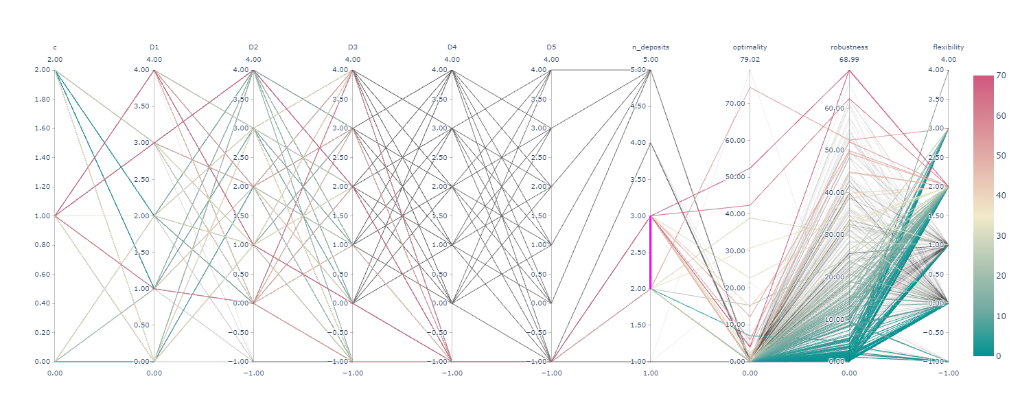
An interactive parallel coordinates plot will also be generated in order to check the relationship between designs in terms of flexibility, robustness, and optimality. Run the file post_process_DOE.py to obtain the following interactive tradespace plot. The interactive .html file will be saved in DOE_results
Please check the following article for more information related to tradespace exploration and design margins
- Scalable Set-Based Design Optimization and Remanufacturing for Meeting Changing Requirements 1
- Optimization of Design Margins Allocation When Making Use of Additive Remanufacturing 2
![]()