This Project is meant to be a theoritical Cource I provide some code but in the abstract way you can readit to understand the concept we refer to some reference in this notebook and the most important reference is Hands‑On Machine Learning with Scikit‑Learn, Keras it is amazing book and I recomend every one has an interest in machince learning and Deep learning to read it.
Autoencoders are artificial neural networks capable of learning dense representations
of the input data
what mean by that it's unsuprvised Learning the Goal of this type of learning is to learn hidden structure of data.
These codings typically have a much lower dimensionality ==latent than the input data, making autoencoders useful for dimensionality reduction
Autoencoders also act as feature detectors and pass the output of this model to Neural Network.
Autoencoders are also generative models.
take as input training samples and learn a model the represent of that distribution
example: you could train an autoencoder on pictures of faces, and it would then be able to generate new faces
However, the generated images are usually fuzzy and not entirely realistic
faces generated by generative adversarial networks (GANs) are now so convincing that it is hard to believe that the people they represent do not exist. You can judge so for yourself by visiting https://thispersondoesnotexist.com/, a website that shows faces generated by a recent GAN architecture called StyleGAN.
you can read more about GAN hear http://GAN.com
Autoencoders simply learn to copy their inputs to their outputs. This may sound like a trivial task, but we will see that constraining the network in various ways can make it rather difficult. For example, you can limit the size of the latent representations, or you can add noise to the inputs and train the network to recover the original inputs. These constraints prevent the autoencoder from trivially copying the inputs directly to the outputs, which forces it to learn efficient ways of representing the data. In short, the codings are byproducts of the autoencoder learning the identity function under some constraints
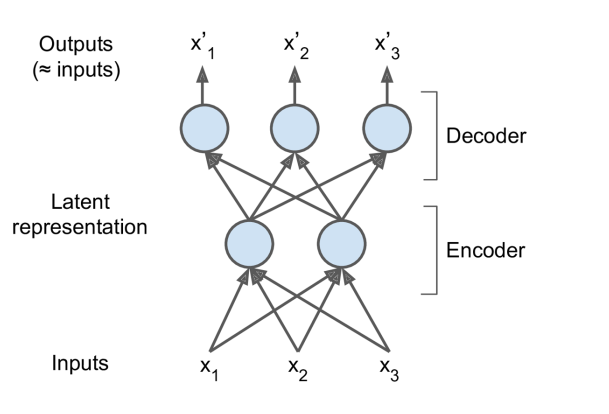
an autoencoder looks at the inputs, converts them to an efficient latent representation, and then spits out some‐ thing that (hopefully) looks very close to the inputs. An autoencoder is always composed of two parts: an encoder (or recognition network) that converts the inputs to a latent representation, followed by a decoder (or generative network) that converts the internal representation to the outputs
As you can see, an autoencoder typically has the same architecture as a Multi-Layer Perceptron except that the number of neurons in the output layer must be equal to the number of inputs. In this example, there is just one hidden layer composed of two neurons (the encoder), and one output layer composed of three neurons (the decoder). The outputs are often called the reconstructions because the autoencoder tries to reconstruct the inputs, and the cost function contains a reconstruction loss that penalizes the model when the reconstructions are different from the inputs. example of reconstruction loss $ min||X_i - X_(output) ||^2$ where $X_i $ is traning example.
Because the internal representation has a lower dimensionality than the input data (it
is 2D instead of 3D), the autoencoder is said to be undercomplete. An undercomplete
autoencoder cannot trivially copy its inputs to the codings, yet it must find a way to
output a copy of its inputs. It is forced to learn the most important features in the
input data (and drop the unimportant ones).
 Let’s see how to implement a very simple undercomplete autoencoder for dimensionality reduction.
in order to force the autoencoder to learn interesting features, we have limited the size of the coding layer,and that what we called undercomplete and the kind of this autoencoders are (basic Autoencoder, Stacked Autoencoder, CNN Autoencoder, RNN Autoencoder)
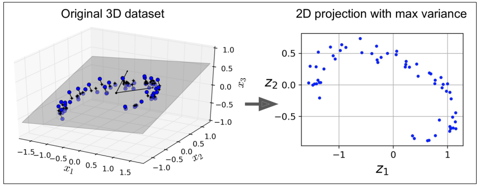
If the autoencoder uses only linear activations and the cost function is the mean squared error mean squre error(MSE), then it ends up performing Principal Component Analysis(PCA)
The following code builds a simple linear autoencoder to perform PCA on a 3D dataset, projecting it to 2D
#code
from tensorflow import keras


encoder = keras.models.Sequential([
            keras.layers.Dense(2, input_shape=[3])
         ])


decoder = keras.models.Sequential([
            keras.layers.Dense(3, input_shape=[2])
         ])


autoencoder = keras.models.Sequential([
              encoder,
              decoder
              ])

autoencoder.compile(loss="mse", optimizer=keras.optimizers.SGD(lr=0.1))
as we can see there is no activation function in all layer and the neuron in output layer is the same as input layer
autoencoder.fit(X_data, X_data) Note that X_data is the input and the targetYou can think of autoencoders as a form of self-supervised learning (i.e., using a supervised learning technique with automatically generated labels, in this case simply equal to the inputs).
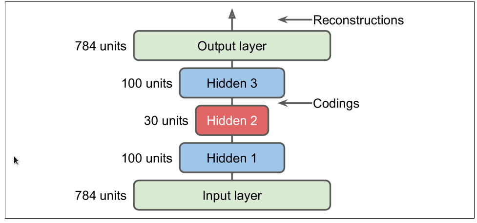
Just like other neural networks we have discussed, autoencoders can have multiple hidden layers. In this case they are called stacked autoencoders
The architecture of a stacked autoencoder is typically symmetrical with regard to the
central hidden layer (the coding layer). To put it simply, it looks like a sandwich. For
example, an autoencoder for MNIST may have 784 inputs,
followed by a hidden layer with 100 neurons, then a central hidden layer of 30 neu‐
rons, then another hidden layer with 100 neurons, and an output layer with 784 neurons.
#code
import tensorflow.keras as keras

stacked_encoder = keras.models.Sequential([
        keras.layers.Flatten(input_shape=[28, 28]),
        keras.layers.Dense(100, activation="selu"),
        keras.layers.Dense(30, activation="selu"),
    ])
stacked_decoder = keras.models.Sequential([
        keras.layers.Dense(100, activation="selu", input_shape=[30]),
        keras.layers.Dense(28 * 28, activation="sigmoid"),
        keras.layers.Reshape([28, 28])
    ])

stacked_ae = keras.models.Sequential([
                stacked_encoder,
                stacked_decoder
             ])

stacked_ae.compile(loss="binary_crossentropy", optimizer=keras.optimizers.SGD(lr=1.5))

history = stacked_ae.fit(X_train, X_train,...)

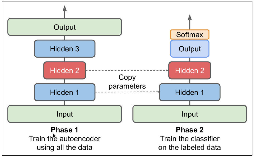
you can use this code to train your modelf you have a large dataset but most of it is unlabeled, you can first train a stacked autoencoder using all the data, then reuse the lower layers to create a neural network for your actual task and train it using the labeled data. For example, Figure shows how to use a stacked autoencoder to perform unsupervised pretraining for a classification neural network. When training the classifier, if you really don’t have much labeled training data, you may want to freeze the pretrained layers (at least the lower ones).
When an autoencoder is neatly symmetrical by symmetrical autoencoder we mean that the encoder layer is as the decoder layer in the inverse way, a common technique is to tie the weights of the decoder layers to the weights of the encoder layers. This halves the number of weights in the model, speeding up training and limiting the risk of overfitting
this is an aowsem technique to use,this come from linear algebra.
if i multiplie matrix
and as we know if the Matrix is Symmetric then the inverse is
the idea if Tying Weights it's depend on the previous explaining the code below show the coustom DenseTranspose layer.
source for multiplie matrix https://www.youtube.com/watch?v=or6C4yBk_SY
#code

import tensorflow as tf
import tensorflow.keras as keras

class DenseTranspose(keras.layers.Layer):
        def __init__(self, dense, activation=None, **kwargs):
            self.dense = dense
            self.activation = keras.activations.get(activation)
            super().__init__(**kwargs)

        def build(self, batch_input_shape):
            self.biases = self.add_weight(name="bias", initializer="zeros",shape=[self.dense.input_shape[-1]])
            super().build(batch_input_shape)
        def call(self, inputs):
            z = tf.matmul(inputs, self.dense.weights[0], transpose_b=True)
            // this function multiplie by the transpose of the layer we pass to the constuctor
            return self.activation(z + self.biases)

dense_1 = keras.layers.Dense(100, activation="selu")
dense_2 = keras.layers.Dense(30, activation="selu")
tied_encoder = keras.models.Sequential([
        keras.layers.Flatten(input_shape=[28, 28]),
        dense_1,
        dense_2
    ])

tied_decoder = keras.models.Sequential([
        DenseTranspose(dense_2, activation="selu"),
        DenseTranspose(dense_1, activation="sigmoid"),
        keras.layers.Reshape([28, 28])
    ])

tied_ae = keras.models.Sequential([tied_encoder, tied_decoder])

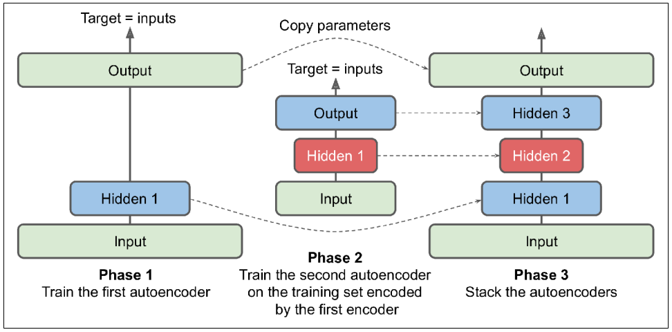
//then you can train this model much fasterRather than training the whole stacked autoencoder in one go like we just did, it is
possible to train one shallow autoencoder at a time, then stack all of them into a single stacked autoencoder (hence the name), as shown in Figure This technique is not used as much these days, but you may still run into papers that talk about “greedy layerwise training,” so it’s good hear about you can search for more information.
convolutional neural networks are far better suited than dense networks to work with images. So if
you want to build an autoencoder for images (e.g., for unsupervised pretraining or dimensionality reduction), you will need to build a convolutional autoencoder
The encoder is a regular CNN composed of convolutional layers and pooling layers.
while decoder do the reverse (upscale the image and reduce its depth back to the original dimensions), and for this you can use transpose convolutional layers (alternatively, you could combine upsampling layers with convolutional layers)
the follwing code show simple Convolutional Autoencoders
#code

import tensorflow as tf
import tensorflow.keras as keras

conv_encoder = keras.models.Sequential([
        keras.layers.Reshape([28, 28, 1], input_shape=[28, 28]),
        keras.layers.Conv2D(16, kernel_size=3, padding="same", activation="selu"),
        keras.layers.MaxPool2D(pool_size=2),
        keras.layers.Conv2D(32, kernel_size=3, padding="same", activation="selu"),
        keras.layers.MaxPool2D(pool_size=2),
        keras.layers.Conv2D(64, kernel_size=3, padding="same", activation="selu"),
        keras.layers.MaxPool2D(pool_size=2)
    ])

conv_decoder = keras.models.Sequential([
        keras.layers.Conv2DTranspose(32, kernel_size=3, strides=2, padding="valid",activation="selu",
        input_shape=[3, 3, 64]),
        keras.layers.Conv2DTranspose(16, kernel_size=3, strides=2, padding="same",activation="selu"),
        keras.layers.Conv2DTranspose(1, kernel_size=3, strides=2, padding="same",activation="sigmoid"),
        keras.layers.Reshape([28, 28])
    ])

conv_ae = keras.models.Sequential([conv_encoder, conv_decoder])If you want to build an autoencoder for sequences, such as time series or text (e.g., for unsupervised learning or dimensionality reduction), then recurrent neural networks may be better suited than dense networks. Building a recurrent autoencoder is straightforward: the encoder is typically a sequence-to-vector RNN which compresses the input sequence down to a single vector. The decoder is a vector-to-sequence RNN that does the reverse.
recurrent_encoder = keras.models.Sequential([
            keras.layers.LSTM(100, return_sequences=True, input_shape=[None, 28]),
            keras.layers.LSTM(30)
        ])

recurrent_decoder = keras.models.Sequential([
            keras.layers.RepeatVector(28, input_shape=[30]),
            keras.layers.LSTM(100, return_sequences=True),
            keras.layers.TimeDistributed(keras.layers.Dense(28, activation="sigmoid"))
        ])

recurrent_ae = keras.models.Sequential([recurrent_encoder, recurrent_decoder])

//Note that we use a RepeatVector layer as the first layer of the decoder, to ensure that its input vector gets fed to the decoder at each time step.There are actually many other kinds of constraints that can be used, including ones that allow the coding layer to be just as large as the inputs, or even larger and the kind of this autoencoders are (Denoising Autoencoders, Sparse Autoencoders)
Another way to force the autoencoder to learn useful features is to add noise to its
inputs, training it to recover the original, noise-free inputs. This idea has been around
since the 1980s (e.g., it is mentioned in Yann LeCun’s 1987 master’s thesis). In a 2008
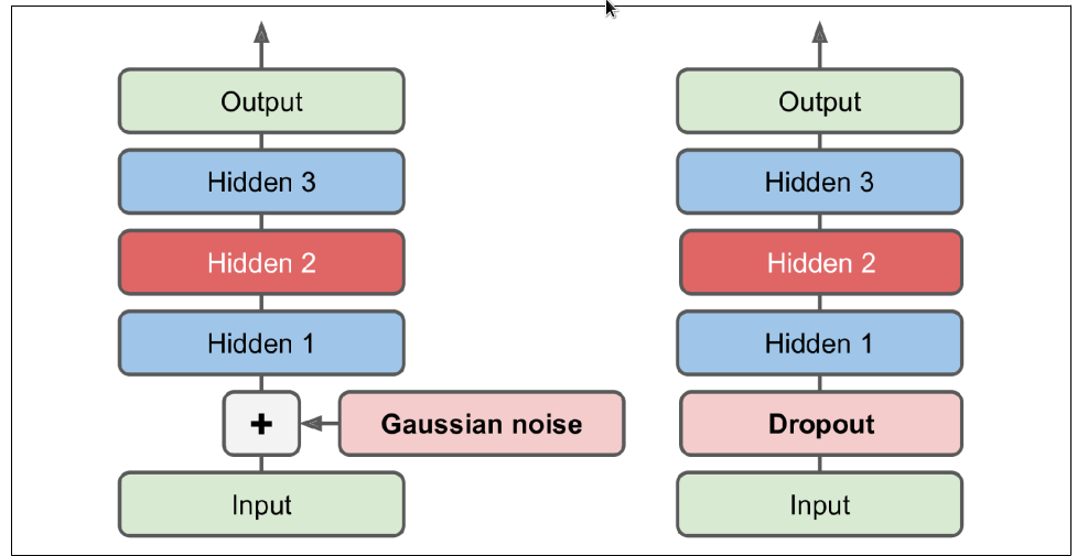
The noise can be pure Gaussian noise added to the inputs, or it can be randomly switched-off inputs, just like in dropout. Figure shows both options.
# code
import tensorflow.keras as keras

// the Dropout noise
dropout_encoder = keras.models.Sequential([
            keras.layers.Flatten(input_shape=[28, 28]),
            keras.layers.Dropout(0.5),
            keras.layers.Dense(100, activation="selu"),
            keras.layers.Dense(30, activation="selu")
        ])
dropout_decoder = keras.models.Sequential([
            keras.layers.Dense(100, activation="selu", input_shape=[30]),
            keras.layers.Dense(28 * 28, activation="sigmoid"),
            keras.layers.Reshape([28, 28])
        ])

dropout_ae = keras.models.Sequential([dropout_encoder, dropout_decoder])

// the Gaussian noise
dropout_encoder = keras.models.Sequential([
            keras.layers.Flatten(input_shape=[28, 28]),
            keras.layers.GaussianNoise(),
            keras.layers.Dense(100, activation="selu"),
            keras.layers.Dense(30, activation="selu")
        ])
dropout_decoder = keras.models.Sequential([
            keras.layers.Dense(100, activation="selu", input_shape=[30]),
            keras.layers.Dense(28 * 28, activation="sigmoid"),
            keras.layers.Reshape([28, 28])
        ])

dropout_ae = keras.models.Sequential([dropout_encoder, dropout_decoder])

//Gaussian and dropout layer thay both active only during the training.Another kind of constraint that often leads to good feature extraction is sparsity: by adding an appropriate term to the cost function, the autoencoder is pushed to reduce the number of active neurons in the coding layer. For example, it may be pushed to have on average only 5% significantly active neurons in the coding layer. This forces the autoencoder to represent each input as a combination of a small number of activations. As a result, each neuron in the coding layer typically ends up representing a useful feature
A simple approach is to use the sigmoid activation function in the coding layer (to
constrain the codings to values between 0 and 1), use a large coding layer and add some
agood source about
we want to penalize the neurons that are too active, or not active enough, by adding a sparsity loss to the cost function.
For example, if we measure that a neuron has an average activation of 0.3, but the target
sparsity is 0.1, it must be penalized to activate less. One approach could be simply
adding the squared error
Given two discrete probability distributions P and Q, the KL divergence between these distributions, noted D KL (P ∥ Q), can be computed
which is the cross-Entropy - Entropy
cross-Entopy :$H(P,Q)=∑_i -P_i log(Q_i) $ and that is the loss function called categorial-crossentropy
Entropy : $ E(P) =∑_i -P_i log(P_i)$ is avery important topic in information theory
In our case, we want to measure the divergence between the target probability
Once we have computed the sparsity loss for each neuron in the coding layer, we sum up these losses and add the result to the cost function. In order to control the relative importance of the sparsity loss and the reconstruction loss, we can multiply the spar‐ sity loss by a sparsity weight hyperparameter. If this weight is too high, the model will stick closely to the target sparsity, but it may not reconstruct the inputs properly, making the model useless. Conversely, if it is too low, the model will mostly ignore the sparsity objective and will not learn any interesting features
Another important category of autoencoders was introduced in 2013 by Diederik
Kingma and Max Welling and quickly became one of the most popular types of
autoencoders called variational autoencoders
They are quite different from all the autoencoders we have discussed so far, in these particular ways:
• They are probabilistic autoencoders, meaning that their outputs are partly determined by chance, even after training (as opposed to denoising autoencoders,which use randomness only during training).

• Most importantly, they are generative autoencoders, meaning that they can generate new instances that look like they were sampled from the training set.
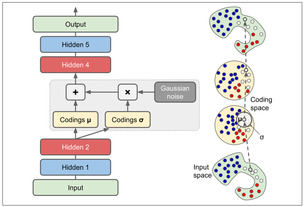
Let’s take a look at how they work. Figure (left) shows a variational autoencoder. You can recognize the basic structure of all autoencoders, with an encoder followed by a decoder (in this example, they both have two hidden layers), but there is a twist: instead of directly producing a coding for a given input, the encoder produces a mean coding μ and a standard deviation σ. The actual coding is then sampled randomly from a Gaussian distribution with mean μ and standard deviation σ. After that the decoder decodes the sampled coding normally. The right part of the diagram shows a training instance going through this autoencoder. First, the encoder pro‐ duces μ and σ, then a coding is sampled randomly (notice that it is not exactly located at μ), and finally this coding is decoded; the final output resembles the training instance.
As you can see in the diagram, although the inputs may have a very convoluted distribution, a variational autoencoder tends to produce codings that look as though they were sampled from a simple Gaussian distribution during training, the cost function pushes the codings to gradually migrate within the coding space (also called the latent space) to end up looking like a cloud of Gaussian points.
One great consequence is that after training a variational autoencoder, you can very easily generate a new instance: just sample a random coding from the Gaussian distribution, decode it
Now, let’s look at the cost function. It is composed of two parts. The first is the usual reconstruction loss that pushes the autoencoder to reproduce its inputs (we can use cross entropy for this, as discussed earlier). The second is the latent loss that pushes the autoencoder to have codings that look as though they were sampled from a simple Gaussian distribution: it is the KL divergence between the target distribution (i.e., the Gaussian distribution) and the actual distribution of the codings. The math is a bit more complex than with the sparse autoencoder, in particular because of the Gaus‐ sian noise, which limits the amount of information that can be transmitted to the coding layer (thus pushing the autoencoder to learn useful features). Luckily, the
equations simplify, so the latent loss can be computed quite simply using
In this equation, ℒ is the latent loss, n is the codings’ dimensionality, and
A common tweak to the variational autoencoder’s architecture is to make the encoder
output
This approach is more numerically stable and speeds up training.
good source for learn more about Variational Autoencoders:
1-Variational autoencoders by JERMY JORDON: https://www.jeremyjordan.me/variational-autoencoders/
2-Understanding Variational Autoencoders (VAEs) by jOSEPH ROCCA: https://towardsdatascience.com/understanding-variational-autoencoders-vaes-f70510919f73
3-Tutorial - What is a variational autoencoder? by JANN ALTOSAAR:https://jaan.io/what-is-variational-autoencoder-vae-tutorial/
# code is for MINST data set

import tensorflow as tf
import tensorflow.keras as keras
import tensorflow.keras.backend as K

class Sampling(keras.layers.Layer):
        def call(self, inputs):
            mean, log_var = inputs
        return K.random_normal(tf.shape(log_var)) * K.exp(log_var / 2) + mean


codings_size = 10
inputs = keras.layers.Input(shape=[28, 28])
z = keras.layers.Flatten()(inputs)
z = keras.layers.Dense(150, activation="selu")(z)
z = keras.layers.Dense(100, activation="selu")(z)
codings_mean = keras.layers.Dense(codings_size)(z) # μ
codings_log_var = keras.layers.Dense(codings_size)(z) # γ
codings = Sampling()([codings_mean, codings_log_var])
variational_encoder = keras.Model(inputs=[inputs], outputs=[codings_mean, codings_log_var, codings])

decoder_inputs = keras.layers.Input(shape=[codings_size])
x = keras.layers.Dense(100, activation="selu")(decoder_inputs)
x = keras.layers.Dense(150, activation="selu")(x)
x = keras.layers.Dense(28 * 28, activation="sigmoid")(x)
outputs = keras.layers.Reshape([28, 28])(x)
variational_decoder = keras.Model(inputs=[decoder_inputs], outputs=[outputs])

_, _, codings = variational_encoder(inputs)
reconstructions = variational_decoder(codings)
variational_ae = keras.Model(inputs=[inputs], outputs=[reconstructions])


latent_loss = -0.5 * K.sum(1 + codings_log_var - K.exp(codings_log_var) - K.square(codings_mean),axis=-1)

variational_ae.add_loss(K.mean(latent_loss) / 784.)

variational_ae.compile(loss="binary_crossentropy", optimizer="rmsprop")
