kd383 / GPML_SLD

Scalable Log Determinants for Gaussian Process Kernel Learning (https://arxiv.org/abs/1711.03481) (NIPS 2017)

Scalable Log Determinants for Gaussian Process Kernel Learning

This repository contains the experiments of the Scalable Log Determinants for Gaussian Process Kernel Learning by Kun Dong, David Eriksson, Hannes Nickisch, David Bindel, Andrew Gordon Wilson. This paper will be appearing at NIPS 2017.

The bibliographic information for the paper is

@inproceedings{dong2017logdet,
  title={Scalable Log Determinants for Gaussian Process Kernel Learning},
  author={Dong, Kun and Eriksson, David and Nickisch, Hannes and Bindel, David and Wilson, Andrew Gordon},
  booktitle={Advances in Neural Information Processing Systems},
  year={2017}
}

Contents

1. Introduction
2. Setup
3. Usage
   1. Hickory Tree Distribution
   2. Natural Sound Modeling
   3. Crime Forecasting
   4. Precipitation Prediction

Introduction

The computation of the log determinant with its derivatives for positive definite kernel matrices appears in many machine learning applications, such as Bayesian neural networks, determinantal point processes, elliptical graphical models, and kernel learning for Gaussian processes (GPs). Its cubic-scaling cost becomes the computational bottleneck for scalable numerical methods in these contexts. Here we propose a few novel linear-scaling approaches to estimate these quantities from only fast matrix vector multiplications (MVMs). Our methods are based on stochastic approximations using Chebyshev, Lanczos, and surrogate models. We illustrate the efficiency, accuracy and flexibility of our approaches with experiments covering

1. Various kernel types, such as square-exponential, Matérn, and spectral mixture.
2. Both Gaussian and non-Gaussian likelihood.
3. Previously prohibitive data size.

Setup

1. Clone this repository
2. Run startup.m

Usage

The code is built with Matlab. In particular, the Lanczos algorithm with reorthogonalization uses ARPACK which comes with Matlab by default. If you are using Octave and require reorthogonalization, replace lanczos_arpack with lanczos_full in cov/apx.m. Fast Lanczos implementation without reorthogonalization is also available by setting ldB2_maxit = -niter. Please check the comments in demos for example.

Hickory Tree Distribution

In this experiment we apply a log-Gaussian Cox model with the RBF kernel and the Poisson likelihood to a point pattern of 703 Hickory tree. The dataset comes from the R package spatstat.

To run this experiment you can use the demo_hickory command. This should take about a minute, and produce the figure below.

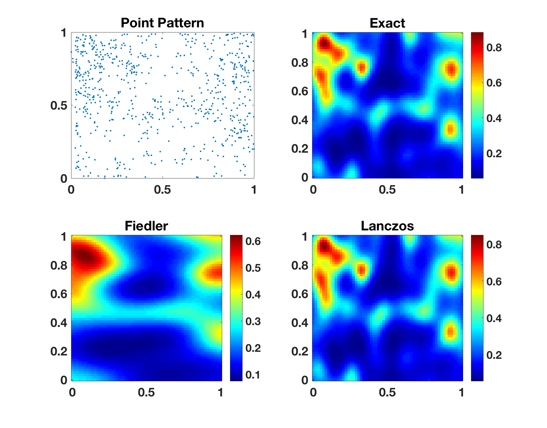
You will see that the Lanczos method produces qualitatively superior prediction than the scaled eigenvalues + Fiedler method. Flexibility is a key advantage of the Lanczos method since it only uses fast MVMs, while scaled eigenvalues method does not directly apply to non-Gaussian likelihoods, hence requires additional approximations.

Natural Sound Modeling

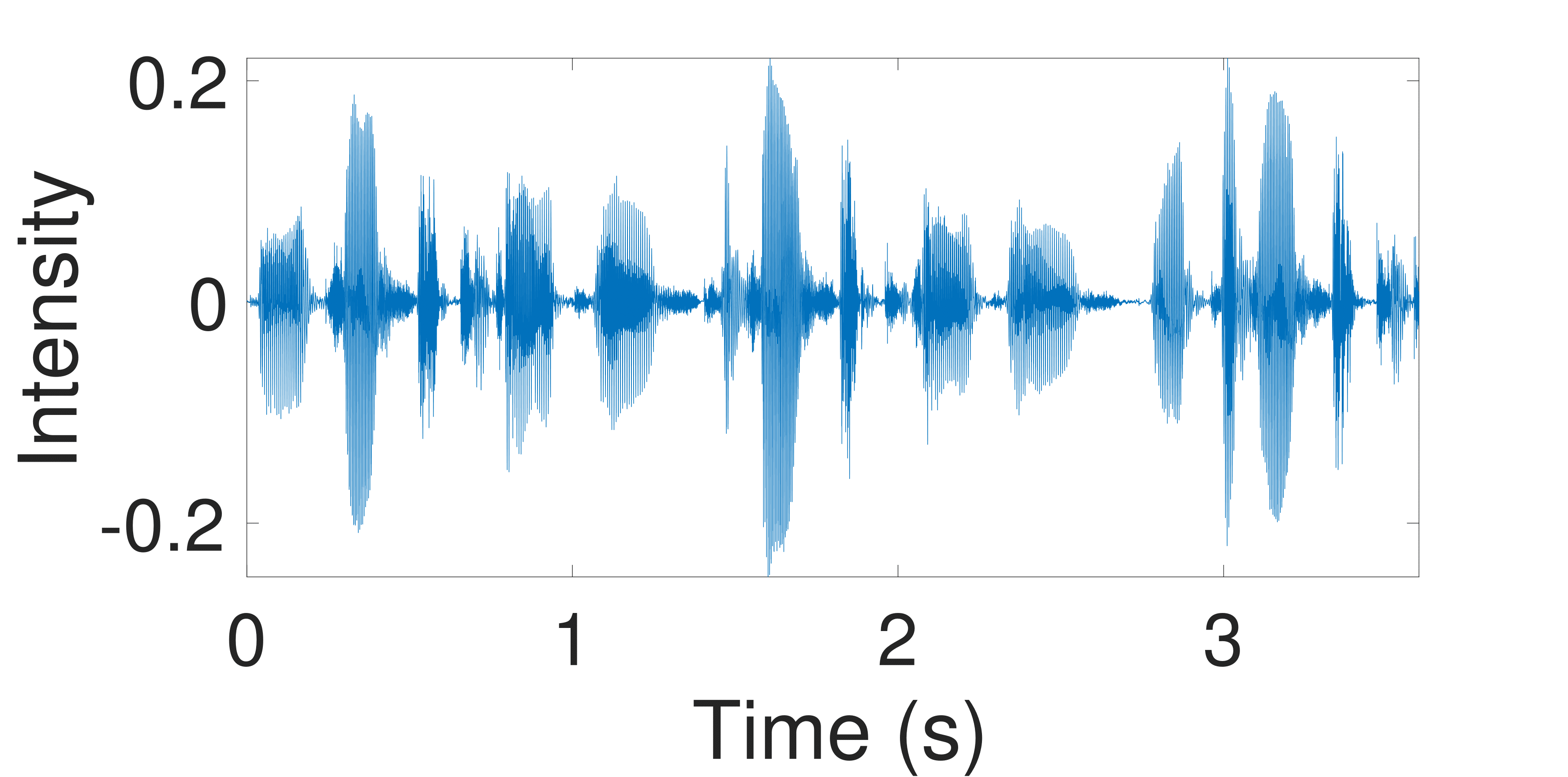
In this experiment we try to recover contiguous missing regions in a waveform with n = 59306 data points. Use the command demo_sound with inputs

1. method: 'lancz' (default), 'cheby', 'ski', 'fitc'
2. ninterp: Number of interpolative grid points. Default: 3000.

Here the accuracy of the prediction is mostly controlled by the number of grid points you use for structured kernel interpolation (SKI). A reasonable range will be between 3000 and 5000. If you run the full experiment setting stored in the data file, you can produce the figure below. As the grid size grows, even the quadratic-scaling cost for scaled eigenvalues method can become prohibitive, but our linear-scaling method remains efficient.

Crime Forecasting

In this experiment we work on the dataset of 233088 assault incidents in Chicago from January 1, 2004 to December 31, 2013. We use the first 8 years for training and try to forecast the crime rate during the last 2 years. For the spatial dimensions, we use the log-Gaussian Cox process model, with the Matérn-5/2 kernel, the negative binomial likelihood, and the Laplace approximation for the posterior; for the temporal dimension we use a spectral mixture kernel with 20 components and an extra constant component.

You can use demo_crime to run this experiment. It takes two arguments:

1. method: 'lancz' (default) for Lanczos method and any other input for scaled eigenvalues method.
2. hyp: Initial hyper-parameters for recovery.

The demo returns the initial and final hyper-parameters for you to reuse. The initial hyper-parameters was originally obtained through a sampling process, which can be time-consuming and may not be a good starting point sometimes. A reasonable initialization is stored in the data file, but you may enable the function spatiotemporal_spectral_init_poisson to get a new one.

Precipitation Prediction

This experiment involves daily precipitation data from the year of 2010 collected from around 5500 weather stations in the US. We fit the data using a GP with RBF kernel. This is a huge dataset with 628474 entries, among which 100000 will be used for testing. As a result, the hyper-parameters recovery part of the experiment takes very long. I recommend using the result stored in the data file for inference and prediction, or run the recovery on a nice desktop.

The command is demo_precip with a single argument method. The default method is Lanczos, and any input other than 'lancz' uses scaled eigenvalues method.