"R package for for the alternate features search"

author: Satoshi Kato (@katokohaku)

Overview

an implementation to R-package of for the alternate features search proposed in the following paper.

S. Hara, T. Maehara, Finding Alternate Features in Lasso, arXiv:1611.05940, 2016.
Complete and original Python code is available from author's github

also introduction slide in Japanese:

Introduction of "the alternate features search" using R

# fit Alternate Lasso model
lasso.cv <- glmnet::cv.glmnet(X, y)
alt1 <- AlternateLasso(X, y, model = lasso.cv$glmnet.fit, rho = lasso.cv$lambda.1se, verbose = FALSE)

plot(alt1, fontSize = 20)

Detail Examples

Installation

You can install the AlternateLassoR package from GitHub.

install.packages("devtools") # if you have not installed "devtools" package
devtools::install_github("hoxo-m/pforeach") # if you have not installed "pforeach" package
devtools::install_github("katokohaku/AlternateLassoR")

The source code for AlternateLassoR package is available on GitHub at

https://github.com/katokohaku/AlternateLassoR.

Data preparation

In this regression example, The Boston Housing Dataset is used. This data set is included in MASS pachage. It is necessary to standardize variables (scaling) before using Lasso Regression because of constraints on the size of the coefficients associated to each variable, such as: $L(\beta):=|X\beta - y|^2+\lambda|\beta|_1$ .

set.seed(1)
require(tidyverse)
require(AlternateLassoR)

data("Boston", package = "MASS")
boston.sc <- scale(Boston)
X <- boston.sc[, -14]
y <- boston.sc[, 14]

Choosing lambda of lasso based on cross-validation

In this example, lambda.1se is used instead of lambda.min, which gives the most regularized model such that error is within one standard error of the minimum, to preserve more alternative variables.

require(glmnet)
lasso.cv <- cv.glmnet(X, y)

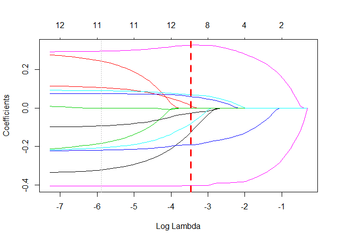
plot(lasso.cv$glmnet.fit, xvar = "lambda")
abline(v=log(lasso.cv$lambda.1se), col="red", lty=2, lwd=3)
abline(v=log(lasso.cv$lambda.min), col="grey", lty=3)

This case, there are 4 potential alternatives (eliminated variables by lasso)

coef.cv.glmnet(lasso.cv, s="lambda.1se")
#> 14 x 1 sparse Matrix of class "dgCMatrix"
#>                         1
#> (Intercept) -4.204596e-16
#> crim        -2.766405e-02
#> zn           1.297615e-02
#> indus        .           
#> chas         5.988494e-02
#> nox         -8.162333e-02
#> rm           3.255561e-01
#> age          .           
#> dis         -1.266486e-01
#> rad          .           
#> tax          .           
#> ptratio     -1.914584e-01
#> black        6.906986e-02
#> lstat       -4.032580e-01

Fit Alternate Lasso model

Currently this package provides only linear regression. For classification tasks with logistic regression, refer to the python code on author's github of the original article.

alt1 <- AlternateLasso(X, y, model = lasso.cv$glmnet.fit, rho = lasso.cv$lambda.1se)
#> [ crim ] has [ 2 ] alternatives
#> [ zn ] has [ 1 ] alternatives
#> [ chas ] has [ 0 ] alternatives
#> [ nox ] has [ 4 ] alternatives
#> [ rm ] has [ 4 ] alternatives
#> [ dis ] has [ 4 ] alternatives
#> [ ptratio ] has [ 4 ] alternatives
#> [ black ] has [ 2 ] alternatives
#> [ lstat ] has [ 4 ] alternatives
summary(alt1)
#>       feature   coef                 
#>  [1,] "crim"    "-0.0276640467240226"
#>  [2,] "zn"      "0.0129761499075482" 
#>  [3,] "indus"   "0"                  
#>  [4,] "chas"    "0.0598849402283941" 
#>  [5,] "nox"     "-0.0816233281893132"
#>  [6,] "rm"      "0.325556124390274"  
#>  [7,] "age"     "0"                  
#>  [8,] "dis"     "-0.126648590185123" 
#>  [9,] "rad"     "0"                  
#> [10,] "tax"     "0"                  
#> [11,] "ptratio" "-0.191458375701974" 
#> [12,] "black"   "0.0690698582439022" 
#> [13,] "lstat"   "-0.403257998979111" 
#> Feature: [ crim ], Coef. = -0.027664, Aiternative: 2
#> 	 Alternate Feature: indus, 	Coef. = -0.007646, Score = 0.000352
#> 	 Alternate Feature: tax, 	Coef. = -0.011056, Score = 0.000320
#> Feature: [ zn ], Coef. = 0.012976, Aiternative: 1
#> 	 Alternate Feature: indus, 	Coef. = -0.003325, Score = 0.000079
#> Feature: [ chas ], Coef. = 0.059885, Aiternative: 0
#> 	 ** No Alternate Features **
#> 
#> 
#> Feature: [ nox ], Coef. = -0.081623, Aiternative: 4
#> 	 Alternate Feature: indus, 	Coef. = -0.058730, Score = 0.001597
#> 	 Alternate Feature: age, 	Coef. = -0.038397, Score = 0.002583
#> 	 Alternate Feature: rad, 	Coef. = -0.006190, Score = 0.003299
#> 	 Alternate Feature: tax, 	Coef. = -0.049461, Score = 0.002098
#> Feature: [ rm ], Coef. = 0.325556, Aiternative: 4
#> 	 Alternate Feature: indus, 	Coef. = -0.123911, Score = 0.045192
#> 	 Alternate Feature: age, 	Coef. = -0.056912, Score = 0.051238
#> 	 Alternate Feature: rad, 	Coef. = -0.024599, Score = 0.052552
#> 	 Alternate Feature: tax, 	Coef. = -0.090012, Score = 0.048811
#> Feature: [ dis ], Coef. = -0.126649, Aiternative: 4
#> 	 Alternate Feature: indus, 	Coef. = 0.030816, Score = 0.007536
#> 	 Alternate Feature: age, 	Coef. = 0.053569, Score = 0.006578
#> 	 Alternate Feature: rad, 	Coef. = 0.043900, Score = 0.007048
#> 	 Alternate Feature: tax, 	Coef. = 0.010294, Score = 0.007957
#> Feature: [ ptratio ], Coef. = -0.191458, Aiternative: 4
#> 	 Alternate Feature: indus, 	Coef. = -0.069774, Score = 0.015847
#> 	 Alternate Feature: age, 	Coef. = -0.028761, Score = 0.017863
#> 	 Alternate Feature: rad, 	Coef. = -0.045261, Score = 0.017254
#> 	 Alternate Feature: tax, 	Coef. = -0.083168, Score = 0.014824
#> Feature: [ black ], Coef. = 0.069070, Aiternative: 2
#> 	 Alternate Feature: indus, 	Coef. = -0.021054, Score = 0.002154
#> 	 Alternate Feature: tax, 	Coef. = -0.025450, Score = 0.002052
#> Feature: [ lstat ], Coef. = -0.403258, Aiternative: 4
#> 	 Alternate Feature: indus, 	Coef. = -0.239885, Score = 0.052420
#> 	 Alternate Feature: age, 	Coef. = -0.221590, Score = 0.056633
#> 	 Alternate Feature: rad, 	Coef. = -0.153345, Score = 0.069401
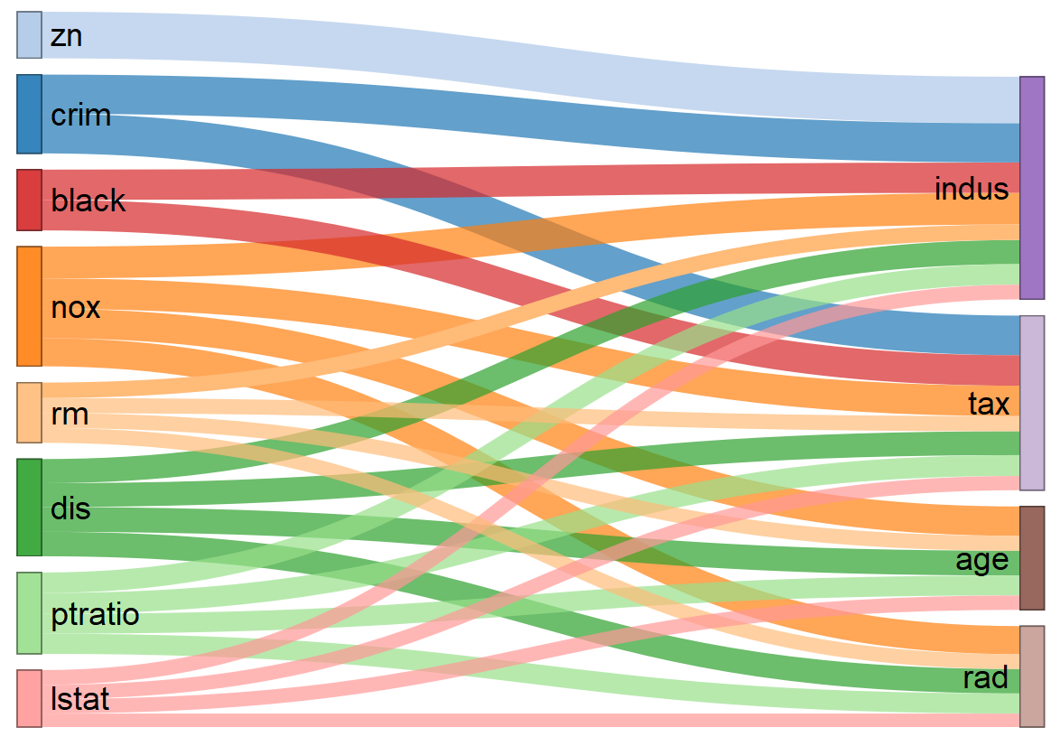
#> 	 Alternate Feature: tax, 	Coef. = -0.214304, Score = 0.058218

Visualize

plots() represents the connections from $\mathrm{var_{original}}$ (left side) to $\mathrm{var_{alternative}}$ (right side) and thier intensity (i.e. $score$ in original paper). Each width of flow corresponds to each score and is displayed as the logarithm of the inverse of its score: $\log_{10}(1 + 1/\mathrm{abs}(score))$.

A wider connection with an alternative indicates that the effect of variable replacement by the alternative could be less severe.

plot(alt1, fontSize = 20)

katokohaku / AlternateLassoR