jwuttke / chebpy

A Python implementation of Chebfun

ChebPy - A Python implementation of Chebfun

Chebpy is a Python implementation of Chebfun.

• For installation details, see INSTALL.rst.
• For implementation notes, see implementation-notes.rst

Demo

For convenience we'll import everything from numpy and matplotlib.

from numpy import *
from matplotlib.pyplot import *
from chebpy import chebfun

The function chebfun behaves in essentially the same way as its Matlab counterpart. A good way to begin is to type:

x = chebfun('x', [0, 10])
x

chebfun column (1 smooth piece)
       interval       length     endpoint values
[       0,      10]        2         0       10
vertical scale =  10

What's happened here is we've instantiated a numerical representation of the identity function on the interval [0,10] and assigned this to a computer variable x. This particular representation has length 2, meaning that it is a degree one polynomial defined via two degrees of freedom (as you would expect of a linear function).

An intuitive set of composition-like operations can now be performed. For instance here is the specification of a function f that oscillates with two modes:

f = sin(x) + sin(5*x)
f

chebfun column (1 smooth piece)
       interval       length     endpoint values
[       0,      10]       58  -4.4e-16    -0.81
vertical scale =   2

The zeros of f can be computed via roots, which behind the scenes is implemented via a recursive subdivision algorithm in which a number of Colleague Matrix eigenvalue sub-problems are solved:

r = f.roots();
r

array([ 0.        ,  0.78539816,  1.04719755,  2.0943951 ,  2.35619449,
        3.14159265,  3.92699082,  4.1887902 ,  5.23598776,  5.49778714,
        6.28318531,  7.06858347,  7.33038286,  8.37758041,  8.6393798 ,
        9.42477796])

By default Chebpy computations are accurate to machine precision, or approximately fifteen digits in double-precision arithmetic (see also UserPrefs). We can verify this for the computed roots of f by typing:

f(r)

array([ -4.44089210e-16,  -4.44089210e-16,  -2.22044605e-16,
        -4.44089210e-16,   2.77555756e-16,  -6.66133815e-16,
         3.88578059e-16,   6.66133815e-16,   2.33146835e-15,
        -4.44089210e-16,   2.10942375e-15,   6.38378239e-16,
        -3.21964677e-15,  -1.55431223e-15,  -2.30371278e-15,
         4.44089210e-15])

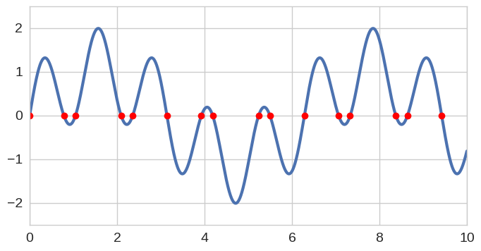
The function and its roots can be plotted together as follows:

f.plot();
plot(r, f(r), 'or');

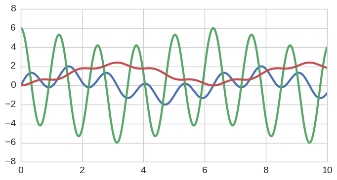
Calculus operations are natively possible with Chebfun objects. For example here is the derivative and indefinite integral of f:

Df = f.diff()
If = f.cumsum()
f.plot(); Df.plot(); If.plot()

One can verify analytically that the exact value of the definite integral here is:

1.2-cos(10)-.2*cos(50)

1.8460783233780296

This matches our numerical integral (via Clenshaw-Curtis quadrature), which is computable in chebpy via the sum command thus:

f.sum()

1.8460783233780327

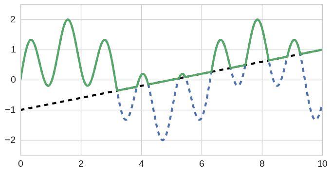
Chebfun is capable of handling certain classes of mathematical nonsmoothness. For example, here we compute the pointwise maximum of two functions, which results in a 'piecewise-smooth' concatenation of twelve individual pieces (in Chebfun & ChebPy terminology this is a collection of 'Funs'). The breakpoints between the pieces (Funs) have been determined by ChebPy in the background by solving the corresponding root-finding problem.

g = x/5 - 1
h = f.maximum(g)
h

chebfun column (12 smooth pieces)
       interval       length     endpoint values
[       0,     3.2]       32  -4.4e-16    -0.36
[     3.2,     3.9]        2     -0.36    -0.23
[     3.9,     4.2]       14     -0.23    -0.15
[     4.2,     5.3]        2     -0.15    0.051
[     5.3,     5.5]       12     0.051    0.092
[     5.5,     6.3]        2     0.092     0.27
[     6.3,       7]       17      0.27     0.39
[       7,     7.5]        2      0.39     0.49
[     7.5,     8.2]       17      0.49     0.65
[     8.2,     8.8]        2      0.65     0.77
[     8.8,     9.3]       15      0.77     0.85
[     9.3,      10]        2      0.85        1
vertical scale =   2    total length = 119

Here's a plot of both f and g, and their maximum, h:

f.plot(linewidth=1, linestyle='--')
g.plot(linewidth=1, linestyle='--')
h.plot()
ylim([-2.5, 2.5]);

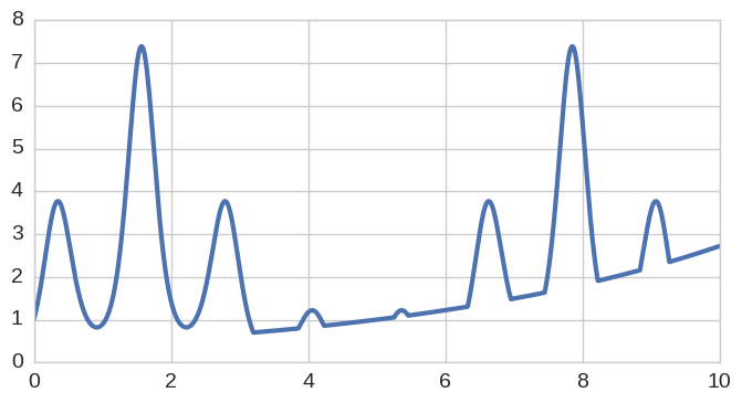
The function h is a further Chebfun representation (Chebfun operations such as this are closures) and thus the same set of operations can be applied as normal. Here for instance is the exponential of h and its integral:

exp(h).plot();

exp(h).sum()

22.090079782676828

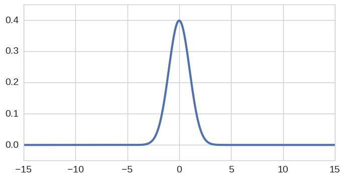
Here's a further example, this time related to statistics. We consider the following Chebfun representation of the standardised Gaussian distribution, using a sufficiently wide interval as to facilitate a machine-precision representation. On this occasion we utlilise a slightly different (but still perfectly valid) approach to construction whereby we supply the function handle (in this case, a Python lambda, but more generally any object in possession of a __call__ attribute) together with the interval of definition.

gaussian = lambda x: 1/sqrt(2*pi) * exp(-.5*x**2)
pdf = chebfun(gaussian, [-15, 15])
pdf.plot()
ylim([-.05, .45]);
title('Standard Gaussian distribution (mean  0, variance 1)');

The integral of any probability density function should be 1, and this is the case for our numerical approximation:

pdf.sum()

0.99999999999999978

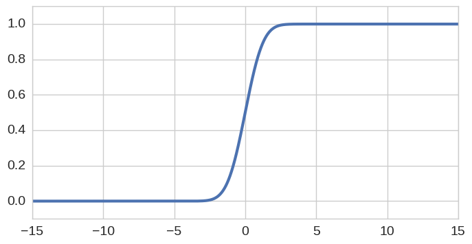
Suppose we wish to generate quantiles of the distribution. This can be achieved as follows. First we form the cumulative distribution function, computed as the indefinite integral (cumsum) of the density:

cdf = pdf.cumsum()
cdf.plot()
ylim([-0.1, 1.1]);

Then it is simply a case of utilising the roots command to determine the standardised score (sometimes known as "z-score") corresponding to the quantile of interest. For example:

print 'quantile    z-score '
print '--------------------'
for quantile in arange(.1, .0, -.01):
    print '  {:2.0f}%       {:+5.3f}'.format(1e2*quantile, (cdf-quantile).roots()[0])

quantile    z-score
--------------------
  10%       -1.282
   9%       -1.341
   8%       -1.405
   7%       -1.476
   6%       -1.555
   5%       -1.645
   4%       -1.751
   3%       -1.881
   2%       -2.054
   1%       -2.326

Other distributional properties are also computable. Here's how we can compute the first four normalised and centralised moments (Mean, Variance, Skew, Kurtosis):

x = pdf.x
m1 = (pdf*x).sum()
m2 = (pdf*(x-m1)**2).sum()
m3 = (pdf*(x-m1)**3).sum() / m2**1.5
m4 = (pdf*(x-m1)**4).sum() / m2**2
print '    mean = {:+.4f}'.format(m1)
print 'variance = {:+.4f}'.format(m2)
print '    skew = {:+.4f}'.format(m3)
print 'kurtosis = {:+.4f}'.format(m4)

    mean = -0.0000
variance = +1.0000
    skew = -0.0000
kurtosis = +3.0000