This package estimates linear models with high dimensional categorical variables and/or instrumental variables.

Installation

The package is registered in the General registry and so can be installed at the REPL with ] add FixedEffectModels.

Benchmarks

The objective of the package is similar to the Stata command reghdfe and the R function felm. The package tends to be much faster than these two options.

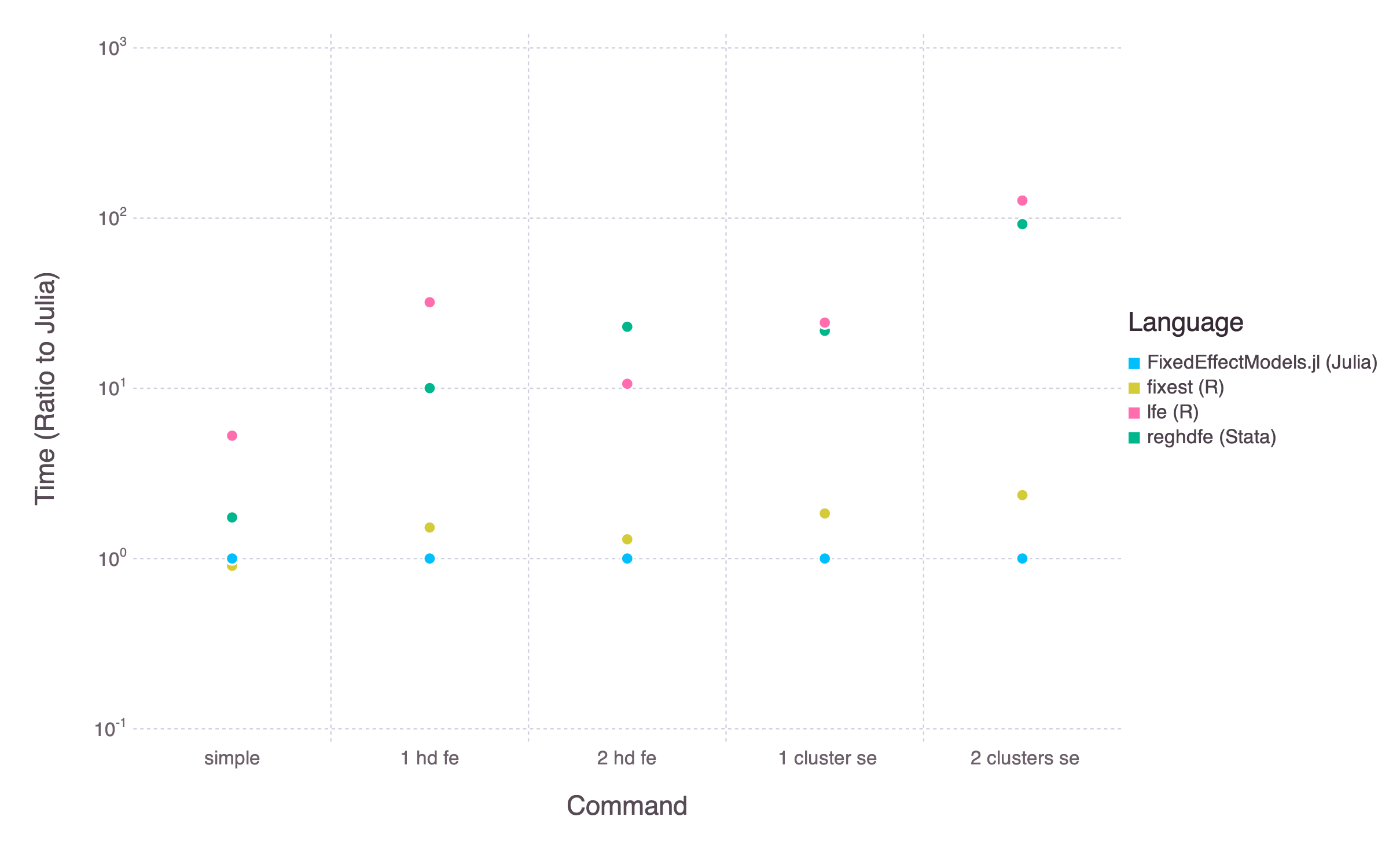
Performances are roughly similar to the newer R function feols. The main difference is that FixedEffectModels can also run the demeaning operation on a GPU (with method = :gpu).

Syntax

using DataFrames, RDatasets, FixedEffectModels
df = dataset("plm", "Cigar")
reg(df, @formula(Sales ~ NDI + fe(State) + fe(Year)), Vcov.cluster(:State), weights = :Pop)
# =====================================================================
# Number of obs:               1380   Degrees of freedom:            32
# R2:                         0.803   R2 Adjusted:                0.798
# F Statistic:              13.3382   p-value:                    0.001
# R2 within:                  0.139   Iterations:                     6
# Converged:                   true
# =====================================================================
#         Estimate  Std.Error  t value Pr(>|t|)   Lower 95%   Upper 95%
# ---------------------------------------------------------------------
# NDI  -0.00526264 0.00144097 -3.65216    0.000 -0.00808942 -0.00243586
# =====================================================================

A typical formula is composed of one dependent variable, exogeneous variables, endogeneous variables, instrumental variables, and a set of high-dimensional fixed effects.
```
dependent variable ~ exogenous variables + (endogenous variables ~ instrumental variables) + fe(fixedeffect variable)
```
High-dimensional fixed effect variables are indicated with the function fe. You can add an arbitrary number of high dimensional fixed effects, separated with +. You can also interact fixed effects using & or *.

For instance, to add state fixed effects use fe(State). To add both state and year fixed effects, use fe(State) + fe(Year). To add state-year fixed effects, use fe(State)&fe(Year). To add state specific slopes for year, use fe(State)&Year. To add both state fixed-effects and state specific slopes for year use fe(State)*Year.
```
reg(df, @formula(Sales ~ Price + fe(State) + fe(Year)))
reg(df, @formula(Sales ~ NDI + fe(State) + fe(State)&Year))
reg(df, @formula(Sales ~ NDI + fe(State)&fe(Year)))              # for illustration only (this will not run here)
reg(df, @formula(Sales ~ (Price ~ Pimin)))
```
To construct formula programatically, use
```
reg(df, term(:Sales) ~ term(:NDI) + fe(:State) + fe(:Year))
```

The option contrasts specifies that a column should be understood as a set of dummy variables:

 reg(df, @formula(Sales ~ Price + Year); contrasts = Dict(:Year => DummyCoding()))

You can specify different base levels

 reg(df, @formula(Sales ~ Price + Year); contrasts = Dict(:Year => DummyCoding(base = 80)))

The option weights specifies a variable for weights
```
 weights = :Pop
```
Standard errors are indicated with the prefix Vcov (with the package Vcov)
```
 Vcov.robust()
 Vcov.cluster(:State)
 Vcov.cluster(:State, :Year)
```
The option save can be set to one of the following: none (default) to save nothing :residuals to save residuals, :fe to save fixed effects. You can access the result with residuals() and fe()
The option method can be set to one of the following: :cpu, :gpu (see Performances below).

Output

reg returns a light object. It is composed of

the vector of coefficients & the covariance matrix (use coef, coefnames, vcov on the output of reg)
a boolean vector reporting rows used in the estimation
a set of scalars (number of observations, the degree of freedoms, r2, etc)
with the option save = true, a dataframe aligned with the initial dataframe with residuals and, if the model contains high dimensional fixed effects, fixed effects estimates (use residuals or fe on the output of reg)

Methods such as predict, residuals are still defined but require to specify a dataframe as a second argument. The problematic size of lm and glm models in R or Julia is discussed here, here, here here (and for absurd consequences, here and there).

You may use RegressionTables.jl to get publication-quality regression tables.

Performances

MultiThreads

FixedEffectModels is multi-threaded. Use the option nthreads to select the number of threads to use in the estimation (defaults to Threads.nthreads()). That being said, multithreading does not usually make a big difference.

GPU

The package has support for GPUs (Nvidia) (thanks to Paul Schrimpf). This can make the package an order of magnitude faster for complicated problems.

To use GPU, run using CUDA before using FixedEffectModels. Then, estimate a model with method = :gpu. For maximum speed, set the floating point precision to Float32 with double_precision = false.

using CUDA, FixedEffectModels
df = dataset("plm", "Cigar")
reg(df, @formula(Sales ~ NDI + fe(State) + fe(Year)), method = :gpu, double_precision = false)

Solution Method

Denote the model y = X β + D θ + e where X is a matrix with few columns and D is the design matrix from categorical variables. Estimates for β, along with their standard errors, are obtained in two steps:

y, X are regressed on D using the package FixedEffects.jl
Estimates for β, along with their standard errors, are obtained by regressing the projected y on the projected X (an application of the Frisch Waugh-Lovell Theorem)
With the option save = true, estimates for the high dimensional fixed effects are obtained after regressing the residuals of the full model minus the residuals of the partialed out models on D using the package FixedEffects.jl

References

Baum, C. and Schaffer, M. (2013) AVAR: Stata module to perform asymptotic covariance estimation for iid and non-iid data robust to heteroskedasticity, autocorrelation, 1- and 2-way clustering, and common cross-panel autocorrelated disturbances. Statistical Software Components, Boston College Department of Economics.

Correia, S. (2014) REGHDFE: Stata module to perform linear or instrumental-variable regression absorbing any number of high-dimensional fixed effects. Statistical Software Components, Boston College Department of Economics.

Fong, DC. and Saunders, M. (2011) LSMR: An Iterative Algorithm for Sparse Least-Squares Problems. SIAM Journal on Scientific Computing

Gaure, S. (2013) OLS with Multiple High Dimensional Category Variables. Computational Statistics and Data Analysis

junyuan-chen / FixedEffectModels.jl