A Python library of common tasks used in the observational radio/mm interferometry data analysis.
The package was developed to aid in the studies of the interstellar medium in high-redshift quasar host galaxies using emission lines, as well as to create publication quality plots.
Download the code, enter the interferopy folder and run
python setup.py install
Or, alternatively, install directly from the repository with
python -m pip install git+https://github.com/mladenovak/interferopy
Two classes, Cube and MultiCube, are defined in cube.py with the goal to speed up the analysis of 2D or 3D data cubes, which are produced by imaging the interferometric data. A collection of helper functions are also available in tools.py. Enable their functionality by importing them.
from interferopy.cube import Cube, MultiCube
import interferopy.tools as iftools
Open a single data cube saved in fits format with
cub = Cube("image.fits")
A 2D map is also considered a 3D cube, only with a single channel. The Cube object gives quick access to useful properties and functions, for example
cub.freqs  # list of frequencies for each channel
cub.vels  # list of velocities for each channel [optionally provide a reference frequency]
cub.rms  # compute and return noise rms in each channel (usual units are Jy/beam)
cub.beam  # beam sizes (resolution in arcsec), e.g., cub.beam["bmaj"]
cub.pixsize  # pixel size in arcsec
Access to the image data is provided via
cub.im  # image, entire data cube
cub.im[px, py, ch]  # a pixel value in a specific channel (one voxel)
cub.im[px, py, :]  # single pixel spectrum along the cube
cub.im[:, :, ch]  # 2D map of a single channel
cub.head  # original fits image header
Converting between pixel and celestial coordinates (usually equatorial coordinate system, in the ICRS or J2000 epoch) is performed with
cub.wcs  # world coordinate system object
px, py = cub.radec2pix(ra, dec)  # pixel to ra/dec coordinates (degrees)
ra, dec = cub.pix2radec(px, py)
ch = cub.freq2pix(freq)  # pixel (channel) to frequency coordinates
freq = cub.pix2freq(ch)
Extract aperture flux density with the spectrum() method, for example
flux, err, _ = cub.spectrum(ra=ra, dec=dec, radius=1.5, calc_error=True)
Omitting the coordinates assumes the central pixel position, which is useful for a quick look at the data, especially in targeted observations, where the source is usually in the phase center. Setting the radius to zero yields a single pixel spectrum. Additional convenience wrapper functions exist (derived from the spectrum() method).
flux = cub.single_pixel_value()  # returns value(s) at the central pixel
flux = cub.aperture_value(ra=ra, dec=dec, radius=0.5)  # integral within a circular aperture of r=0.5"
flux, err = cub.aperture_value(ra=ra, dec=dec, radius=0.5, calc_error=True)
To find the best aperture size that encompasses the entire source, one can search for a saturation point in the curve of growth (cumulative flux density as a function of aperture radius). Obtain it with the growing_aperture() method. This operates on a single channel only (must set the freq or the channel parameter). The same function implements the ability to compute azimuthally averaged radial profile.
r, flux, err, _ = cub.growing_aperture(ra=ra, dec=dec, freq=freq, maxradius=5, calc_error=True)
r, profile, err, _ = cub.growing_aperture(ra=ra, dec=dec, freq=freq, calc_error=True, profile=True)
Again, convenience wrapper functions exist (derived from the growing_aperture() method).
r, flux = cub.aperture_r()  # use the central pixel, the first channel, and the maxradius of 1" by default
r, profile = cub.profile_r()
During the imaging process (e.g., using CASA task tclean), several cubes are produced, which all pertain to the same dataset and the same observed source. The MultiCube is a container, a dictionary-like class that can hold multiple cubes simultaneously. This class also defines functions that operate on multiple cubes, such as the primary beam correction or the rasidual scaled aperture integration. Loading the MultiCube object is performed with
mcub = MultiCube("image.fits")
If a specific naming convention is used, it will load automatically other available cubes in the same directory, such as the image.dirty.fits, image.residual.fits, image.pb.fits, and so on. This behavior can be overriden, and the cubes can be loaded manually
 mcub = MultiCube("image.fits", autoload_multi=False)  # open the first map
 # mcub = MultiCube()  # alternatively, intialize an empty container
 # mcub.load_cube("/somewhere/cube.fits", "image")
 mcub.load_cube("/elsewhere/cube.dirty.fits", "dirty")
 mcub.load_cube("/elsewhere/cube.residual.fits", "residual")
Specific cubes are accessed via their keys:
mcub.loaded_cubes  # list of loaded cubes
cub = mcub["image"]  # return a Cube object
cub = mcub.cubes["image"]  # same as above
Analogous to spectrum() and growing_aperture() methods available for a Cube object, the MultiCube object has spectrum_corrected() and growing_aperture_corrected(). These methods perform aperture integration that takes into account the ill-defined hybrid units of the cleaned maps. They require loaded image, residual, and dirty cubes (best to have the pb cube as well).
flux, err, tab = mcub.spectrum_corrected(ra=ra, dec=dec, radius=1.5, calc_error=True)
r, flux, err, tab = mcub.growing_aperture_corrected(ra=ra, dec=dec, maxradius=5, calc_error=True)
These methods perform both the residual scaling correction, and the primary beam correction (can be turned off with apply_pb_corr=False). The tab will contain a Table object with additional technical information, such as the aperture integrated values from individual cubes, the clean-to-dirty beam ratio, number of pixels or beams in the aperture, and so on.
Additional helper functions are defined in tools.py, for example
iftools.sigfig(1.234, digits=3)  # rounds to 3 significant digits yielding 1.23
iftools.calcrms(cub.im)  # calculate noise rms of the input array
iftools.gausscont(x, cont, amp, freq0, sigma)  # Gaussian on top of a constant continuum profile
Various converter functions are defined here, for example
width_ghz = iftools.kms2ghz(width_kms, freq_ghz)  # channel width in km/s to GHz at the reference frequency
fwhm = iftools.sig2fwhm(sigma)  # convert Gaussian sigma to FWHM
kpc_per_arcsec = iftools.arcsec2kpc(z)  # 1 arcsec to kiloparsecs using concordence cosmology
ra, dec = iftools.sex2deg(ra_hms, dec_dms)  # sexagesimal coordinates h:m:s and d:m:s (strings) to degrees
Additionally, there are several methods used for dust continuum calculations: blackbody() - Planck's law, dust_lum() - compute dust luminosity, dust_sobs() - compute observed flux density of dust. A method to compute the surface brightness temperature of radio observations: surf_temp(). A method to stack different positions in a single 2D map: stack2d(), and others.
Several specialized tasks and helper functions for data reduction in CASA are located in casatools.py and casatools_vla_pipe.py.
Usage of Cube and MultiCube classes, and their methods, are demonstrated on an ALMA dataset of a high-redshift quasar host galaxy J1342+0928, nicknamed Pisco for short. The galaxy host was observed across multiple ALMA bands between 100 and 400 GHz, targeting numerous atomic and molecular emission lines. The results and the method details are published in Novak et al. (2019) and Bañados et al. (2019). For more technical details, see also Novak et al. (2020), where a similar analysis was performed on a larger sample of galaxies.
For the following demonstration, the high resolution data targeting the [CII] atomic fine structure line is used. Data cubes are located in the data folder. The complete code used to generate the paper quality figures, which are shown below, is available in the examples.py.
-
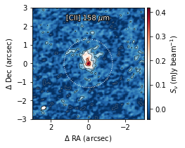
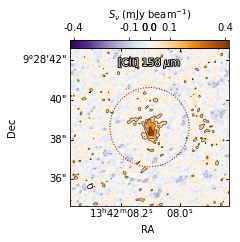
Plot the integrated [CII] line emission centered on the given coordinate. Overlay logarithmic contours, the clean beam (in the bottom left corner), and the aperture circle. The second plot is in a different style with lin-log scaling, wcs axes (also works for continuum maps), and is more accessible to people with colour-blindness.
-
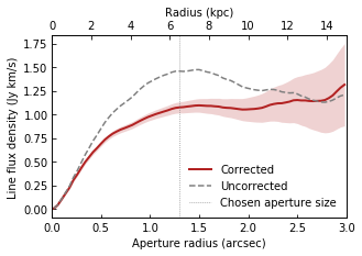
Plot the curve of growth extracted from the above map. Scale the units to line flux density (Jy km/s) and provide a physical distances axis. The residual scaling correction accounts for a non-negligible 35% systematic error.
-
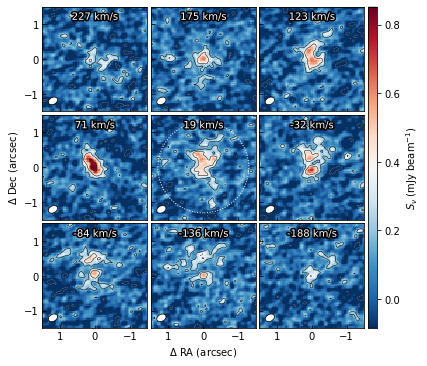
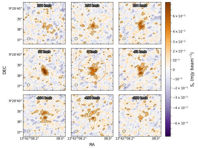
Plot channel maps around the peak line emission (set to be at velocity of 0 km/s). The grid size is easily changed to include more or fewer panels.
-
Or, again, in lin-log scaling and wcsaxes.
-
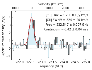
Plot the aperture integrated spectrum extracted from the above cube. Perform residual scaling correction. Fit a Gaussian plus a continuum to estimate the line parameters.
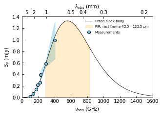
- Fit a modified black body emission to the observed dust continuum emission points. The code is available in dust_continuum_fitting.py. Takes into account the cosmic microwave background heating and contrast. Free fitting parameters are the dust mass, the dust temperature, and the spectral emissivity (slope beta), or a subsample of those. The dust mass affects the overall scaling, the temperature affects the peak position, and beta affects the Rayleigh-Jeans tail slope. The integral below the fitted curve is then converted to star formation rate.
-
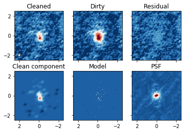
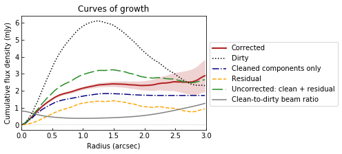
Plot various maps generated during the cleaning process. The cleaned map is the sum of the residual map (units of Jansky per dirty beam, which is the PSF) and the clean component map (units of Jansky per clean beam, which is a Gaussian), and therefore suffers from ill-defined units. Residual scaling method correct for this issue by estimating the clean-to-dirty beam ratio (epsilon).
-
Plot the curves of growth from various maps and show the residual scaling correction in effect.
-
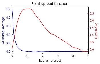
Show the profile (azimuthal average) and the curve of growth (cumulative) of the dirty beam (the PSF). The resolution in the map can be defined to be the FWHM of the PSF profile. Note how the cumulative integral of the dirty beam approaches zero at large radii, causing the units in the residual map to become undefined (Jy / dirty beam).
-
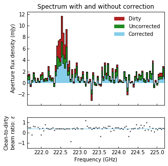
Plot the aperture integrated spectrum derived from multiple maps. Use the high signal-to-noise channels (those with line emission) to fix the clean-to-dirty beam ratio for all channels.
Interferopy includes an implementation of the Findclumps algorithm used by Walter+2016 to find line emitters in ASPECS (https://ui.adsabs.harvard.edu/abs/2016ApJ...833...67W/abstract). At its core, Findclumps simply convolves the cube with boxcar kernels of various sizes, and run sextractor on the created image to find "clumps". It does so on the original and inverted cubes, enabling the user to estimate which detections are real or not. It groups "clumps" by frequency and spatial distance, at the discretion of the user.
To run findlcumps, you will need to have sextractor installed (which can be done via an astroconda environment : https://astroconda.readthedocs.io/en/latest/package_manifest.html), and have a local "default.sex" file in the folder where you run the interferopy-findclumps script. You can either copy your generic default.sex that comes as part of sextractor of modify it to optimise the search for "clumps" in the cube.
Example usage:
from interferopy.cube import Cube
cube = Cube('absolute_path/filename')
cube.findclumps_full(output_file='./output_directory/file_prefix')
kernels= np.arange(3, 20, 2),sextractor_param_file = 'default.sex',
clean_tmp=True, min_SNR=3,delta_offset_arcsec=2,delta_freq=0.1)
cat_Neg = np.loadtxt('./output_directory/file_prefix_clumpsN_minSNR_0_cropped.cat')
cat_Pos = np.loadtxt('./output_directory/file_prefix_clumpsP_minSNR_0_cropped.cat')
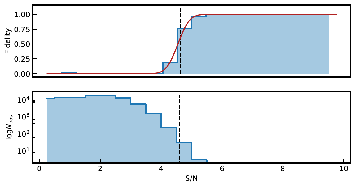
sn_threshold = iftools.fidelity_selection(cat_negative=cat_Neg, cat_positive=cat_Pos, i_SN=5, fidelity_threshold=0.6,
plot_name='./clumps/fidelity_selection_FINDCLUMPS.pdf')
candidates = cat_Pos[np.where(cat_Pos[:,5]>sn_threshold)[0]]
The resulting fidelity selection plot should look like this:
Enjoy one pisco coctail, surrounded by dust, bubbling with CO, and with a twist of CNO elements!

MIT License, Copyright (c) 2020 Mladen Novak