Arthur Samuel described it as: "the field of study that gives computers the ability to learn without being explicitly programmed."

1. Supervised Learning
2. Unsupervised Learning
Predict class or value label
Basically supervised learning is a learning in which we teach or train the machine using data which is well labeled that means some data is already tagged with the correct answer.
1. Regression
2. Classification

In statistical modeling, regression analysis is a set of statistical processes for estimating the relationships between a dependent variable and one or more independent variables.The output variable in regression is numerical (or continuous).
Given a picture of a person, we have to predict their age on the basis of the given picture

-
The purple dots are the points(Original points) on the graph. Each point has an x-coordinate and a y-coordinate.
-
The blue line is our prediction line(we just assume a prediction line). This line contains the predicted points.
-
The red line between each purple point and the prediction line are the errors. Each error is the distance from the point to its predicted point.
y=Mx+B, where M is the slope of the line and B is y-intercept of the line.

Where:

1. ŷi – the value estimated by the regression line

2. ȳ (y bar) – the mean value of a sample
The regression sum of squares describes how well a regression model represents the modeled data. A higher regression sum of squares indicates that the model does not fit the data well.

Where:

1. Yi – the value in a sample

2. ȳ (y bar) – the mean value of a sample
The total sum of squares quantifies the total variation in a sample.

r-squared shows how well the data fit the regression model (the goodness of fit).

Where:
    1. SS(regression) is the sum of squares due to regression (explained sum of squares)
    2. SS(total) is the total sum of squares
In the best case, the modeled values exactly match the observed values, which results in SSR = 0 and R-Squared = 1. A baseline model, which always predicts ȳ , will have R-Squared = 0, Models that have worse predictions than this baseline will have a negative R-Squared.
R-squared increases every time you add an independent variable to the model. The R-squared never decreases, not even when it’s just a chance correlation between variables. A regression model that contains more independent variables than another model can look like it provides a better fit merely because it contains more variables.
Adjusted R-squared is used to compare the goodness-of-fit for regression models that contain differing numbers of independent variables.

n = the sample size

k = the number of independent variables in the regression equation
  1. Simple Linear Regression
  2. Multiple Linear Regression
  3. Polynomial Regression
  4. Support Vector for Regression (SVR)
  5. Decision Tree Regression
  6. Random Forest Regression
Linear regression is a statistical approach for modelling relationship between a dependent variable with a given set of independent variables.
Simple linear regression is an approach for predicting a response (dependent variables) using a single feature(independent variable).
y = βo + β*x

here,
   1. y is the predicted value or the dependent variable for any given value of the independent variable (x).
   2. βo is the intercept, the predicted value of y when the x is 0.
   3. β is the regression coefficient – how much we expect y to change as x increases.
   4. x is the independent variable ( the variable we expect is influencing y).
- All-in
- Backward Elimination
- Forward Selection
- Bidirectional Elimination
- Score Comparison
Backward elimination is a feature selection technique while building a machine learning model. It is used to remove those features that do not have a significant effect on the dependent variable or prediction of output.
Step-1: Firstly, We need to select a significance level to stay in the model. (SL=0.05)

Step-2: Fit the complete model with all possible predictors/independent variables.

Step-3: Choose the predictor which has the highest P-value, such that.

If P-value >SL, go to step 4.
Else Finish, and Our model is ready.
Step-4: Remove that predictor.

Step-5: Rebuild and fit the model with the remaining variables.
import statsmodels.formula.api as sm
def backwardElimination(x, sl):
    numVars = len(x[0])
    for i in range(0, numVars):
        regressor_OLS = sm.OLS(y, x).fit()
        maxVar = max(regressor_OLS.pvalues).astype(float)
        if maxVar > sl:
            for j in range(0, numVars - i):
                if (regressor_OLS.pvalues[j].astype(float) == maxVar):
                    x = np.delete(x, j, 1)
    regressor_OLS.summary()
    return x

SL = 0.05
X_opt = X[:, [0, 1, 2, 3, 4, 5]]
X_Modeled = backwardElimination(X_opt, SL)import statsmodels.formula.api as sm
def backwardElimination(x, SL):
numVars = len(x[0])
temp = np.zeros((50,6)).astype(int)
for i in range(0, numVars):
regressor_OLS = sm.OLS(y, x).fit()
maxVar = max(regressor_OLS.pvalues).astype(float)
adjR_before = regressor_OLS.rsquared_adj.astype(float)
if maxVar > SL:
for j in range(0, numVars - i):
if (regressor_OLS.pvalues[j].astype(float) == maxVar):
temp[:,j] = x[:, j]
x = np.delete(x, j, 1)
tmp_regressor = sm.OLS(y, x).fit()
adjR_after = tmp_regressor.rsquared_adj.astype(float)
if (adjR_before >= adjR_after):
x_rollback = np.hstack((x, temp[:,[0,j]]))
x_rollback = np.delete(x_rollback, j, 1)
print (regressor_OLS.summary())
return x_rollback
else:
continue
regressor_OLS.summary()
return x
SL = 0.05
X_opt = X[:, [0, 1, 2, 3, 4, 5]]
X_Modeled = backwardElimination(X_opt, SL)
Now let us have a brief look at the parameters of the OLS summary.
-
R square – It tells about the goodness of the fit. It ranges between 0 and 1. The closer the value to 1, the better it is. It explains the extent of variation of the dependent variables in the model. However, it is biased in a way that it never decreases(even on adding variables).
-
Adj Rsquare – This parameter has a penalising factor(the no. of regressors) and it always decreases or stays identical to the previous value as the number of independent variables increases. If its value keeps increasing on removing the unnecessary parameters go ahead with the model or stop and revert.
-
F statistic – It is used to compare two variances and is always greater than 0. It is formulated as v12/v22. In regression, it is the ratio of the explained to the unexplained variance of the model.
-
AIC and BIC – AIC stands for Akaike’s information criterion and BIC stands for Bayesian information criterion Both these parameters depend on the likelihood function L.
-
Skew – Informs about the data symmetry about the mean.
-
Kurtosis – It measures the shape of the distribution i.e.the amount of data close to the mean than far away from the mean.
-
Omnibus – D’Angostino’s test. It provides a combined statistical test for the presence of skewness and kurtosis.
-
Log-likelihood – It is the log of the likelihood function.

This image shows the preferred relative values of the parameters.
Backward Elimination with p-values only Implementation
Backward Elimination with p-values and Adjusted R Squared in NoteBook
Polynomial Regression is a form of linear regression in which the relationship between the independent variable x and dependent variable y is modeled as an nth degree polynomial. Polynomial regression fits a nonlinear relationship between the value of x and the corresponding conditional mean of y, denoted E(y |x)
y = a + b1x + b2x^2 +....+ bnx^n
Implementation of Polynomial Regression (Python) in Jupyter Notebook
In simple regression we try to minimise the error rate. While in SVR we try to fit the error within a certain threshold.
- Kernel: The function used to map a lower dimensional data into a higher dimensional data.
- Hyper Plane: In SVM this is basically the separation line between the data classes. Although in SVR we are going to define it as the line that will will help us predict the continuous value or target value
- Boundary line: In SVM there are two lines other than Hyper Plane which creates a margin . The support vectors can be on the Boundary lines or outside it. This boundary line separates the two classes. In SVR the concept is same.
- Support vectors: This are the data points which are closest to the boundary. The distance of the points is minimum or least.
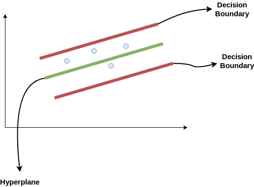
Y = wx+b (equation of hyperplane)
wx+b= +a
wx+b= -a
-a < Y- wx+b < +a
Our main aim here is to decide a decision boundary at ‘a’ distance from the original hyperplane such that data points closest to the hyperplane or the support vectors are within that boundary line.
Medium : Support Vector Regression Or SVR
Implementing Support Vector Regression (SVR) in Python Jupyter Notebook
Decision tree builds regression or classification models in the form of a tree structure. It breaks down a dataset into smaller and smaller subsets while at the same time an associated decision tree is incrementally developed. The final result is a tree with decision nodes and leaf nodes
The core algorithm for building decision trees called ID3 by J. R. Quinlan which employs a top-down, greedy search through the space of possible branches with no backtracking. The ID3 algorithm can be used to construct a decision tree for regression by replacing Information Gain with Standard Deviation Reduction.
- Root Node: It represents entire population or sample and this further gets divided into two or more homogeneous sets.
- Splitting: It is a process of dividing a node into two or more sub-nodes.
- Decision Node: When a sub-node splits into further sub-nodes, then it is called decision node.
- Leaf/Terminal Node: Nodes do not split is called Leaf or Terminal node.
- Pruning: When we remove sub-nodes of a decision node, this process is called pruning. You can say opposite process of splitting.
- Branch / Sub-Tree: A sub section of entire tree is called branch or sub-tree.
- Parent and Child Node: A node, which is divided into sub-nodes is called parent node of sub-nodes whereas sub-nodes are the child of parent node.


Best Article On Decision Tree Regression
Decision trees are sensitive to the specific data on which they are trained. If the training data is changed the resulting decision tree can be quite different and in turn the predictions can be quite different. Also Decision trees are computationally expensive to train, carry a big risk of overfitting, and tend to find local optima because they can’t go back after they have made a split. To address these weaknesses, we turn to Random Forest :) which illustrates the power of combining many decision trees into one model.
A Random Forest is an ensemble technique capable of performing both regression and classification tasks with the use of multiple decision trees and a technique called Bootstrap and Aggregation, commonly known as bagging. The basic idea behind this is to combine multiple decision trees in determining the final output rather than relying on individual decision trees.
An Ensemble method is a technique that combines the predictions from multiple machine learning algorithms together to make more accurate predictions than any individual model. A model comprised of many models is called an Ensemble model.

1. Boosting.
2. Bootstrap Aggregation (Bagging).
Boosting refers to a group of algorithms that utilize weighted averages to make weak learners into stronger learners. Boosting is all about “teamwork”.In boosting as the name suggests, one is learning from other which in turn boosts the learning.
Bootstrap refers to random sampling with replacement. Bootstrap allows us to better understand the bias and the variance with the dataset. Bootstrap involves random sampling of small subset of data from the dataset. Bagging makes each model run independently and then aggregates the outputs at the end without preference to any model.
Random forest is a bagging technique and not a boosting technique. The trees in random forests are run in parallel. There is no interaction between these trees while building the trees.
It operates by constructing a multitude of decision trees at training time and outputting the class that is the mode of the classes (classification) or mean prediction (regression) of the individual trees.


1. It is one of the most accurate learning algorithms available. For many data sets, it produces a highly accurate classifier.
2. It runs efficiently on large databases.
3. It can handle thousands of input variables without variable deletion.
4. It gives estimates of what variables that are important in the classification.
5. It generates an internal unbiased estimate of the generalization error as the forest building progresses.
6. It has an effective method for estimating missing data and maintains accuracy when a large proportion of the data are missing.
1. Random forests have been observed to overfit for some datasets with noisy classification/regression tasks.

2. For data including categorical variables with different number of levels, random forests are biased in favor of those attributes with more levels.
Therefore, the variable importance scores from random forest are not reliable for this type of data.
Determine data patterns/groupings
Unsupervised learning is the training of machine using information that is neither classified nor labeled and allowing the algorithm to act on that information without guidance. Here the task of machine is to group unsorted information according to similarities, patterns and differences without any prior training of data.
Suppose it is given an image having both dogs and cats which have not seen ever.
Thus the machine has no idea about the features of dogs and cats so we can’t categorize it in dogs and cats.
But it can categorize them according to their similarities, patterns, and differences i.e., we can easily categorize the above picture into two parts.
First first may contain all pics having dogs in it and second part may contain all pics having cats in it.
1. Clustering
2. Association
1. Hierarchical clustering
2. K-means clustering
3. K-NN (k nearest neighbors)
4. Principal Component Analysis
5. Singular Value Decomposition
6. Independent Component Analysis