Electric Brew

NEEFC Energy Efficiency Project for Austin Street Brewery

Quick Links

Welcome to the Electric Brew Project! Below you'll find quick links to key documents and resources that provide in-depth information about various aspects of our data pipeline and infrastructure:

Data Dictionary: Delve into our detailed data dictionary, which offers a complete overview of all the tables, fields, and their data types within the project.
Data Lineage and Parquet Tips: Understand the lineage of our data and get practical tips for working with Parquet files, ensuring effective data management and analysis.
ERD and DuckDB Usage: Access our Entity-Relationship Diagram (ERD) for a visual representation of our data model, along with guidelines for leveraging DuckDB for your data queries and storage needs.
Data Pipeline Functions: Explore the comprehensive list of functions utilized in our data pipeline, detailing their purposes and usage.

Project Team

Sean Sullivan (@seanmainer)
Joseph Nelson Farrell (@nfarrell011)
James Parkington (@jparkington)

Stakeholders

Luke Truman: New England Environmental Finance Center (NEEFC), Sustainability Coordinator
Will Fisher: Austin Street Brewery, Co-founder & CEO

Story

Austin Street Brewery, a thriving craft beer brewery situated in Maine, is at an exciting stage of its growth trajectory. With expansion comes opportunities for innovation, and the brewery's energy infrastructure is a prime example. Currently, energy consumption is measured through seven different electricity meters, each tied to various operational facets of the brewery, from brewing and packaging to maintaining a welcoming atmosphere in the tasting room.

As a forward-thinking establishment, Austin Street Brewery has already made strides towards sustainability by sourcing 15% of their energy from solar power and are keen to understand how they might increase this proportion effectively. With multiple supplier contracts and the complexity that comes with sustainable energy sources, there exists a unique opportunity to streamline their energy management practices.

In collaboration with Luke Truman from the New England Environmental Finance Center (NEEFC), whom has a proven track record in aiding craft beverage producers in enhancing energy efficiency and environmental sustainability, Austin Street Brewery aims to leverage data science for the following objectives:

Operational cost mapping to understand which meters should power which equipment.
Benchmarking against industry standards to identify areas for improvement.
Analysis of total energy usage to compare the cost-efficiency of solar versus conventional suppliers.
Unbiased peak hour and supplier recommendations based on unsupervised machine learning models.

Installation & Usage

This project utilizes Conda for managing dependencies and environments. Conda enables the creation of isolated environments that can house specific versions of packages, making it easier to manage complex projects. It's particularly well-suited for Python-based data science projects, ensuring that all dependencies are compatible and can be easily installed or removed.

Setting Up the Environment

For the shortest path to getting up and running, you can simply run the command below, which will create the Conda environment and ensure the pathing is set up properly for subsequent commands and ad hoc querying.

make setup

Note that each script containing a plot saves a PNG file in the .fig directory after being closed by the user.

The entire ETL process is ready for you upon cloning the repo. However, you can reproduce the scraping, curating, and modeling steps with the command below.

make etl

All Makefile Commands

Each of these commands can be called from the CLI with the keyword construction make {command}.

Environment Management with Conda

create-env: Creates a new Conda environment using the environment.yml file.
remove-env: Removes the Conda environment, deleting all installed packages and dependencies.
set-pythonpath: Sets the PYTHONPATH environment variable for the current Conda environment.
setup: Composite command that creates the environment and sets PYTHONPATH.
update-env: Updates the Conda environment as per the environment.yml file.

ETL Pipeline

etl: Initiates the ETL pipeline, preparing the data for analytics.

Initial Exploratory Data Analysis (EDA)

eda1: Executes EDA scripts for kWh distribution, usage patterns, and energy spikes.
eda2: Runs EDA scripts for visualizing kWh usage by period, time, and location.

Operational Cost Mapping

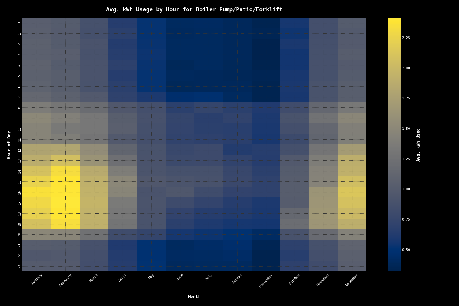
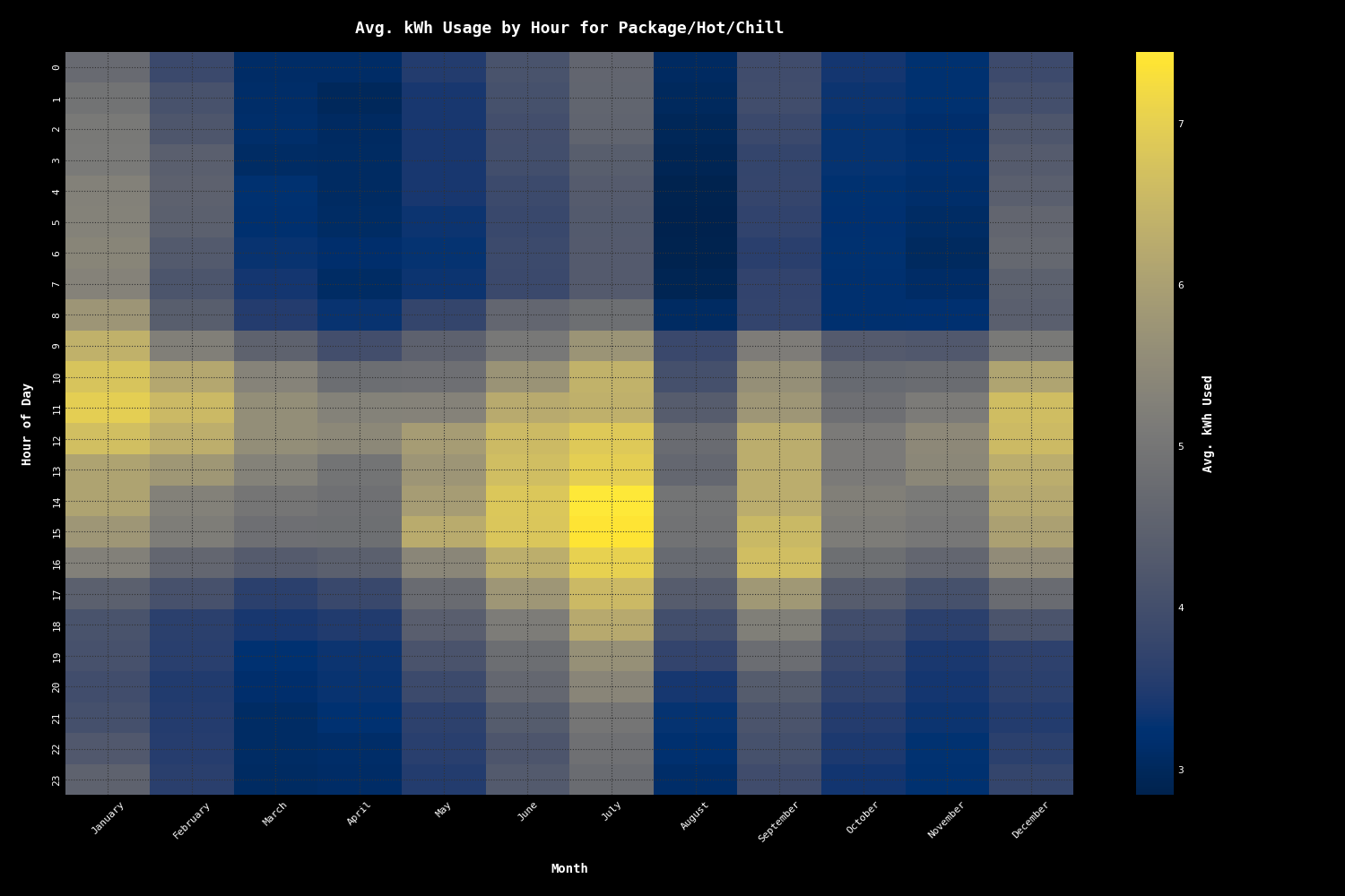
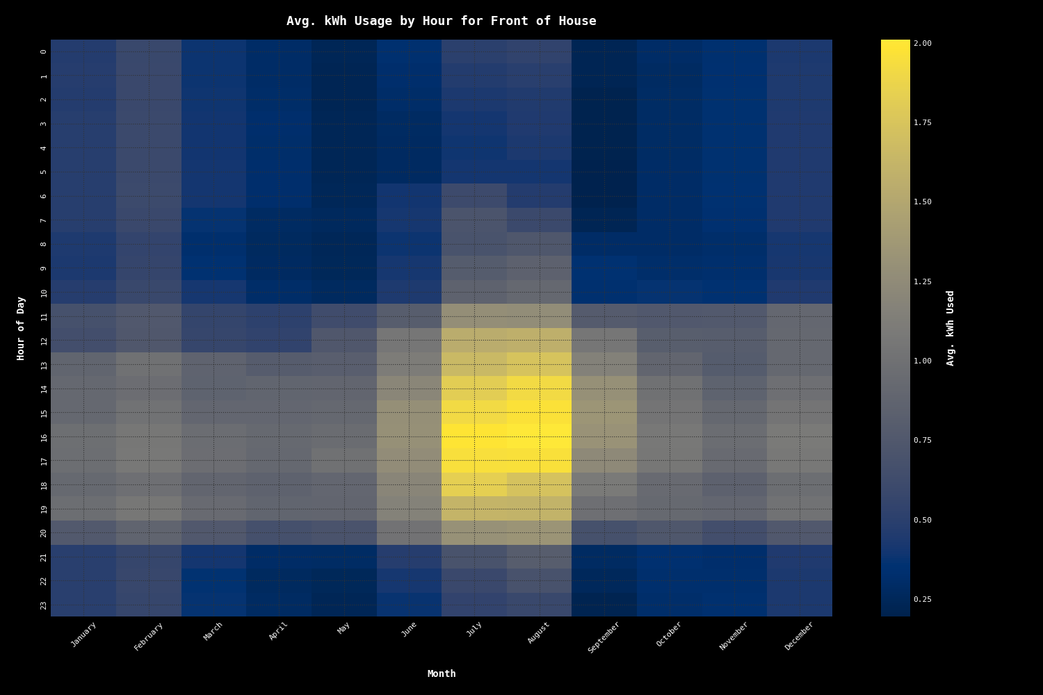
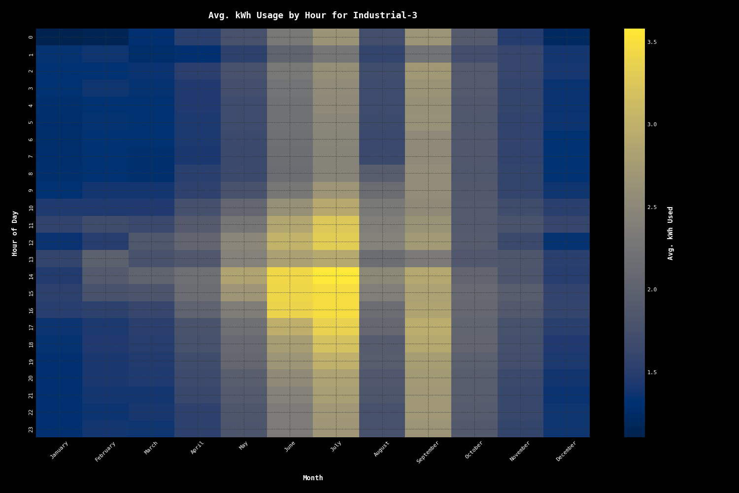
ss01: Generates a line chart of total kWh usage by operational area over time.
ss02: Creates heatmaps for kWh usage by hour and month for each operational area.
ss-all: Executes all scripts in 'Operational Cost Mapping' sequentially.

Energy Usage Analysis

nf01: Visualizes total energy usage at Austin Street Brewery over the course of the dataset.
nf02: Visualizes energy usage by different time intervals.
nf03: Produces a breakdown of energy usage by generation type (solar vs. conventional).
nf04: Produces a summary visual of cost per kWh across generation types.
nf05: Generates projections for solar power costs for Austin Street Brewery.
nf-all: Executes all scripts in 'Energy Usage Analysis' sequentially.

Peak Hour & Supplier Modeling

jp01: Visualizes the relationship between kWh and Total Cost.
jp02: Visualizes hourly variation of kWh usage by month.
jp03: Visualizes average cost by period over time.
jp04: Applies anomaly detection using Isolation Forest.
jp05: Visualizes heatmap of high correlations among numeric columns.
jp06: Applies feature selection using LASSO.
jp07: Fits a Linear Regression model and visualizes results.
jp08: Fits a Random Forest model and visualizes predictions.
jp09: Compares cross-validation R² scores across models.
jp10: Performs SLSQP optimization and visualizes results.
jp11: Visualizes percentage changes in categorical values after optimization.
jp-all: Executes all scripts in 'Peak Hour & Supplier Modeling' sequentially.

All Analysis

analysis: Executes each of the analysis sections in order of the project's objectives.

Analysis

In the Analysis section, we delve into the interconnected themes of operational efficiency, cost management, and sustainable energy use at Austin Street Brewery. Our approach reveals the complex interplay between energy consumption patterns, cost implications, and the potential of renewable energy sources. We uncover insights into how different operational areas contribute to overall energy usage, identifying specific periods and practices that drive up costs.

This analysis is not just about pinpointing areas of high consumption but also understanding the underlying factors contributing to these patterns. We then explore the financial and environmental aspects of the brewery's energy mix, evaluating the current balance between conventional and solar energy and projecting future scenarios. The culmination of our analysis offers strategic recommendations, leveraging advanced modeling to propose optimizations in energy usage and supplier relationships.

Throughout this section, our focus remains on providing a holistic view that blends operational practicality with a vision for sustainable growth, offering Austin Street Brewery a roadmap to not only reduce costs but also enhance their environmental footprint.

Exploratory Data Analysis

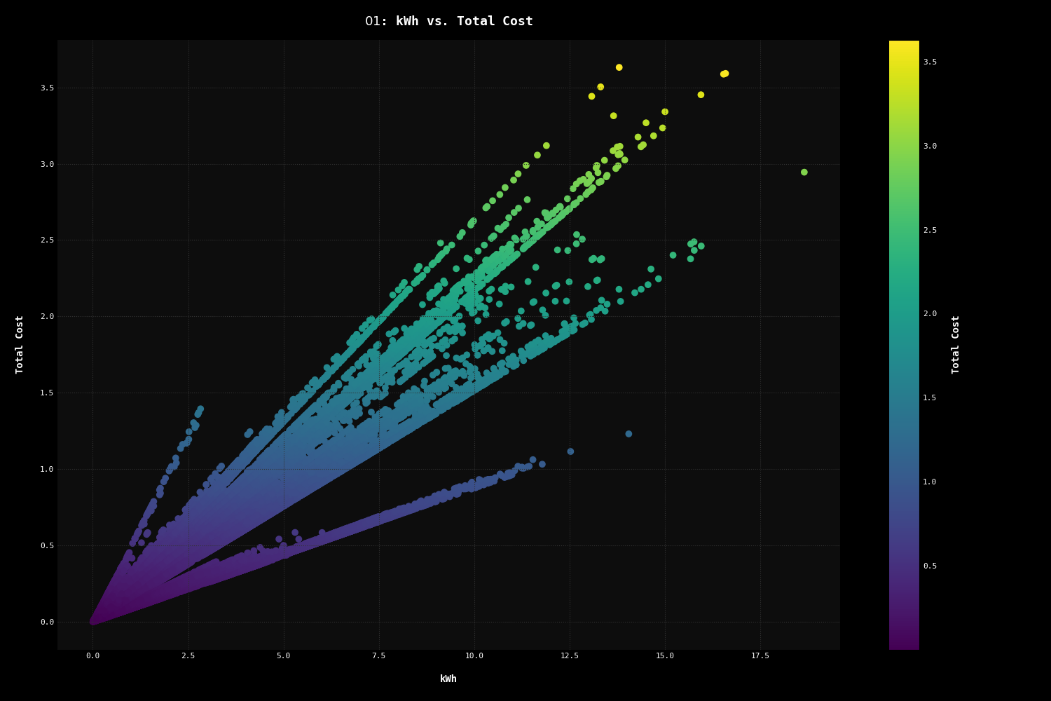
make jp01

Our analysis of the relationship between kilowatt-hours (kWh) and total cost is pivotal in strategizing for maximum energy efficiency at the lowest possible cost, a relationship that underpins each of our project's objectives. The data, encompassing over 301,281 entries, indicates considerable variability in both energy usage and cost. The average kWh usage is 0.849 with a standard deviation of 1.309, and the average total cost is $0.14 per reading with a standard deviation of $0.23. This variability is underscored by the right-skewed distribution for both metrics, pointing to infrequent but significant spikes in energy usage and cost.

A key insight from this analysis is the strong positive correlation of 0.926 between kWh and total cost. This correlation suggests a general trend where increased energy usage leads to higher costs. It also reveals the intricacies of this relationship, influenced by the static rates from CMP, suppliers, and Ampion. The pattern-driven, striated nature observed in the scatter plot indicates that the cost dynamics are not simply linear but are affected by these structured rate tiers.

These insights offer a significant opportunity for strategic operational adjustments, particularly in targeting periods where high energy usage does not proportionally equate to high costs. Identifying these cost-efficient periods, possibly due to favorable rate structures or operational efficiencies, can lead to substantial savings.

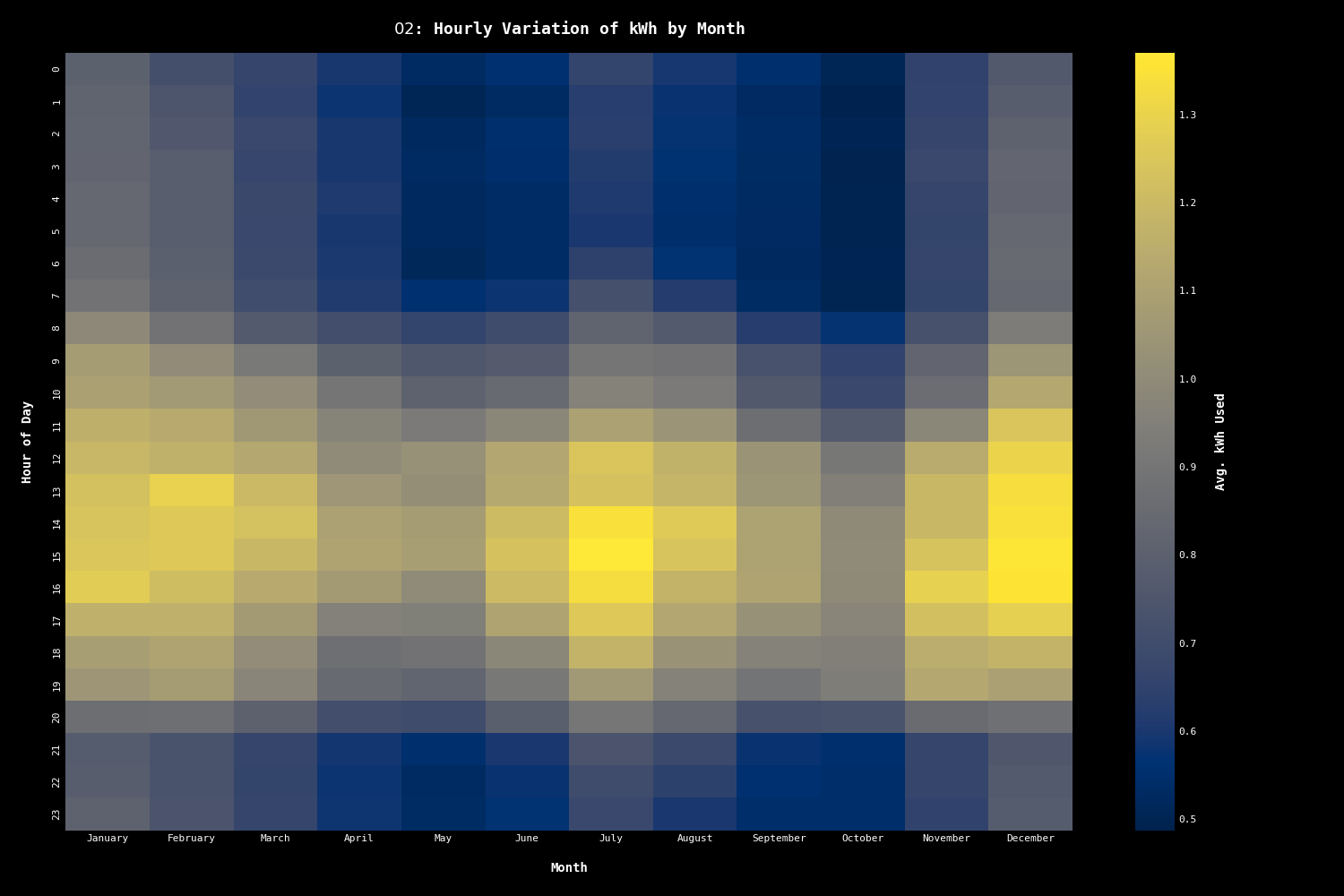
make jp02

Following our examination of the kWh versus total cost relationship, the analysis of hourly kWh usage by month uncovers its stark seasonal variations, reflecting the brewery's heightened energy demands during the colder months, likely exacerbated by the need for heating during Maine's harsh winters. That necessity had become even more pronounced in the context of COVID-19, which we'll explore in later charts.

From the data, we observe that the energy usage peaks in the winter months, with January and December recording the highest average kWh usage at 0.99 and 1.01 respectively. This trend is indicative of increased heating requirements and possibly a higher operational pace during the holiday season. In contrast, the milder months of April and May show lower energy consumption, averaging at 0.78 and 0.73 kWh. The hourly breakdown within each month further reveals a consistent pattern of energy usage ramping up during the morning hours, peaking in the midday to early afternoon, and then gradually declining towards the night. This pattern aligns with typical operational hours and suggests that most energy-intensive activities occur during the day, tapering off as the brewery closes for the night.

Aligning energy-intensive processes with periods of lower kWh usage, especially during off-peak hours, could save on operational costs, assuming variable rates are available for Austin Street to opt into. Implementing energy storage solutions could also be beneficial, allowing the brewery to store energy during off-peak hours for use during peak demand times.

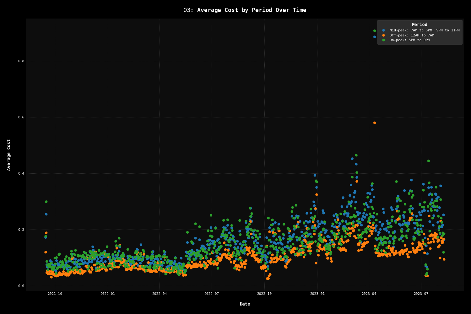
make jp03

Building on our earlier analyses, the scatter plot depicting average cost by period over time at Austin Street Brewery underscores the nuances in their energy usage, particularly under the lens of peak and off-peak hours. A key observation from the data is the brewery's tendency towards higher energy usage during peak hours, as reflected in the average costs: $0.16 for mid-peak, $0.10 for off-peak, and $0.15 for on-peak hours. This pattern is pivotal, as it suggests that a straightforward transition to a variable rate plan, without adjusting operational practices, might not be as beneficial as hoped.

In short, the concentration of data points during peak hours in the scatter plot indicates that the brewery's current energy-intensive activities align with generally more expensive energy periods. This presents an opportunity for strategic operational adjustments, such as rescheduling certain activities to off-peak hours, which could lead to more substantial cost savings. This approach, however, needs to be balanced with the practicalities of brewery operations, ensuring that any changes do not adversely affect productivity or product quality.

Operational Cost Mapping

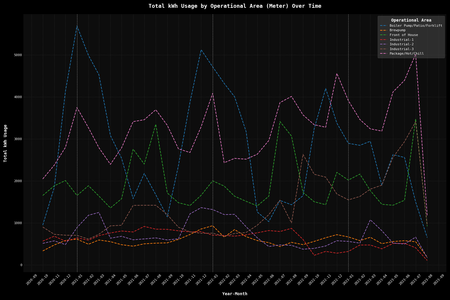
make ss01

A standout observation in this chart is the significant power usage in areas associated with heating and cooling. The 'Boiler Pump/Patio/Forklift' area at Fox St. (represented in blue) shows marked spikes in power consumption during winter months. These spikes correlate with periods of COVID-19 when outdoor seating was prevalent, necessitating the use of patio heaters. Despite a reduction in outdoor seating, the energy usage remains high, likely driven by the boiler's continued operation for brewing processes.

Similarly, the 'Front of House' area (shown in green) exhibits increased energy usage during peak summer months, an interesting inverse to the Patio line. This trend likely reflects the heightened demand for air conditioning during this period.

And finally, in the 'Industrial-3' line (highlighted in brown), there is a significant uptick in kWh usage starting in the summer of 2022. Upon consultation with stakeholders, we learned that this increase was due to the installation of a large walk-in cooler at the Industrial Way location.

These insights point to potential areas for energy efficiency improvements and cost savings. For instance, exploring more energy-efficient heating solutions for the patio area and optimizing the usage of cooling systems in the Front of House could yield some benefits, since they seem to be the major drivers of energy consumption at these two locations.

make ss02

Building upon our previous analysis, which highlighted significant power usage in areas associated with heating and cooling, the newly generated heatmaps not only further substantiate some of those initial observations, but they also showcase how inter-related operational patterns can be for different areas of the business.

Boiler Pump/Patio/Forklift: Consistent with our previous findings, the heatmap for this area shows pronounced energy usage in the winter months, especially during evenings. This aligns with the operational hours of patio heaters used during the COVID-19 period, when outdoor seating was essential.
Front of House: Also echoing our earlier observation, this area's energy consumption peaks in the summer, highlighting the significant use of air conditioning. The focused usage during these warmer months, particularly in business hours, emphasizes the need for cooling systems to maintain a comfortable environment, and presents an opportunity for exploring more energy-efficient cooling solutions.
Package/Hot/Chill: This area demonstrates a relatively stable energy usage throughout the year with a notable decrease in late summer, assumedly due to the installation of a walk-in cooler at Industrial Street no longer necessitating the same degree of chilling for this Fox Street meter.
Industrial-3: A marked increase in energy usage is observed during the summer months. This surge corresponds with our previous finding of the new walk-in cooler installation at the Industrial Way location, underscoring the impact of such capital improvements on the brewery's energy needs.

Energy Usage Analysis

make nf01

The data on total energy usage shows a gradual increase in kilowatt-hours over the years, with the lowest monthly usage recorded in October 2020 at 6,966.84 kWh and the peak in August 2023 at 15,031.38 kWh. This trend suggests a growing operational scale that mimics the brewery's expansion into more space over that period.

A key observation is the notable increase in average energy usage following the introduction of solar power in September 2022. Before the Ampion partnership, the average monthly energy usage was around 11,003.24 kWh. Post the solar power transition, this average rose to approximately 12,216.07 kWh. This increase can be attributed to several factors, including expanded operations, more energy-intensive processes, and some seasonal variation.

make nf02

In looking more closely at the energy supply by generation type, the data distinctly shows that during summer months, the brewery derives a substantial portion of its energy from solar power, with peaks in solar energy usage notably in September at 87.4%. The surrounding months approximate a 75% distribution, which is in alignment with the brewery's original apportioning agreement for their solar credit allocation.

However, during winter months, the reliance on solar energy diminishes significantly, with the lowest solar energy usage recorded in December at merely 8.5%. This seasonal variance is characteristic of Maine's climate, where solar energy generation is less efficient during shorter, cloudier winter days. The stark contrast in energy sourcing between summer and winter months reflects the natural limitations of solar power in the northeastern United States but also highlights an opportunity for Austin Street to optimize its energy management.

Given the higher solar energy production in summer, if the brewery were ability to bank energy credits, perhaps by enhancing solar energy storage capabilities, that could potentially yield better performance even in less ideal conditions.

make nf03

While embracing solar energy is a significant step towards sustainability, it currently comes at a higher monetary cost. The total energy costs over time show considerable variability, with a mean monthly cost of about $1,773.40. Breaking down the costs by generation type, solar energy consistently incurs higher expenses, with a mean monthly cost of $1,461.84, compared to conventional sources at $1,074.25. This consistent trend, despite the variability in costs, might be influenced by the efficiency and technology of solar power, particularly in Maine's seasonal climate.

The higher mean monthly cost for solar energy highlights the current economic challenges of sustainable energy solutions. It's important to consider the broader context, including the assumed long-term savings and environmental benefits of solar power. These factors, beyond the immediate financial comparison, may influence the overall viability of solar energy for the brewery. However, without in-depth knowledge of long-term economic impacts and potential incentives, assessing the financial feasibility of solar power for Austin Street Brewery requires a more comprehensive analysis.

make nf04

In this analysis, we explore a hypothetical scenario where all of Austin Street's power is sourced from solar energy. The actual vs. projected energy costs reveal a clear trend that follows from the previous charts—switching entirely to solar power would have led to higher expenses for the brewery. Over the analyzed period, the average actual cost per month stands at about $2,362.32, whereas the projected costs under a full solar regime average around $2,524.36.

Interestingly, the cost per kWh for solar energy averages at $0.224, with a relatively stable standard deviation of $0.025. This consistency contributes to higher projected costs, reaffirming that, under current conditions and pricing models, solar energy is more expensive per unit than the brewery's existing energy mix.

The analysis becomes particularly insightful when examining the percentage differences between actual and projected costs, especially in significant months. For instance, in December 2022, the cost difference reaches a substantial 50.31%, and in January 2023, it stands at 36.41%. These figures underscore the substantial financial impact that a full shift to solar energy could have during months with higher energy demands.

In summary, while the transition to solar energy aligns with sustainability goals, it currently presents a considerable cost increase for Austin Street Brewery, particularly in high-demand months. This analysis highlights the importance of a balanced approach, where solar energy complements rather than completely replaces conventional energy sources. It also underscores the need for further exploration into cost-effective solar solutions, potential subsidies, and incentives that could make a full transition more financially viable in the future.

Peak Hour & Supplier Modeling

Based on our previous sections, some patterns have started to emerge:

Heating and cooling processes incur significant energy costs.
Partnership with Ampion, though sustainable, appears financially steeper compared to conventional energy sources.
Austin Street Brewery's main operational activities are concentrated within specific hours.

However, the complexity and intentional obscurity in the data from energy providers necessitate a deeper dive. To carry this out, we apply a series of unsupervised machine learning models to the data, including anomaly detection, multicollinearity analysis, feature selection, regression techniques, and optimization techniques. These models serve a dual purpose:

To rip through the intricate layers of the dataset, revealing underlying patterns and inefficiencies.
To validate and enhance our initial insights by identifying the most impactful variables, uncovering hidden operational patterns, and ensuring robust and generalizable predictions.

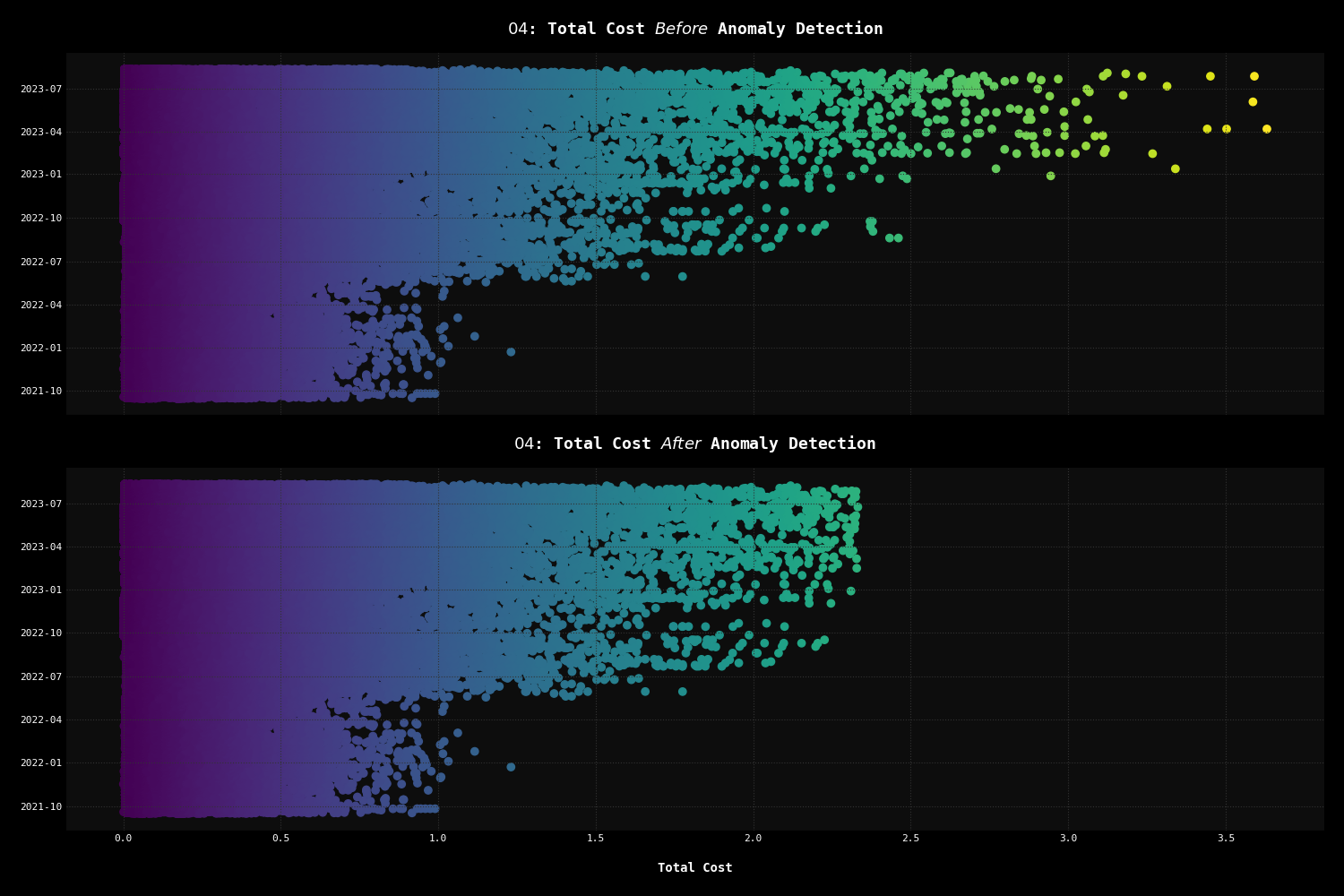
make jp04

The first step in our series of unsupervised models is to apply an Isolation Forest algorithm to trim the outliers from our total_cost data, removing anomalies from the dataset. This is crucial because these outliers can muddle our analysis, especially considering the clear patterns we've started to see, like the high costs associated with heating, cooling, and solar energy from Ampion.

Before Anomaly Detection: The initial dataset, with nearly a half-million entries, shows a wide range of total_cost values (min: $0.00, max: $3.63) with a mean of $0.1389 and a relatively high standard deviation of $0.2340. This high variance indicates significant fluctuations in energy costs, possibly reflecting occasional spikes in energy usage or pricing anomalies from Austin Street's suppliers.
After Anomaly Detection: After applying IsolationForest, the mean total_cost slightly decreases to $0.1371, and the standard deviation is reduced slightly to $0.2239, indicating a more uniform dataset. The maximum cost value notably drops to $2.33, suggesting that the removed anomalies were indeed significantly higher than typical cost values.
Number of Detected Anomalies: With 220 anomalies detected and removed, the dataset becomes more representative of the brewery's regular energy cost patterns. This reduction in extreme values should allow for more accurate analysis in subsequent machine learning models.

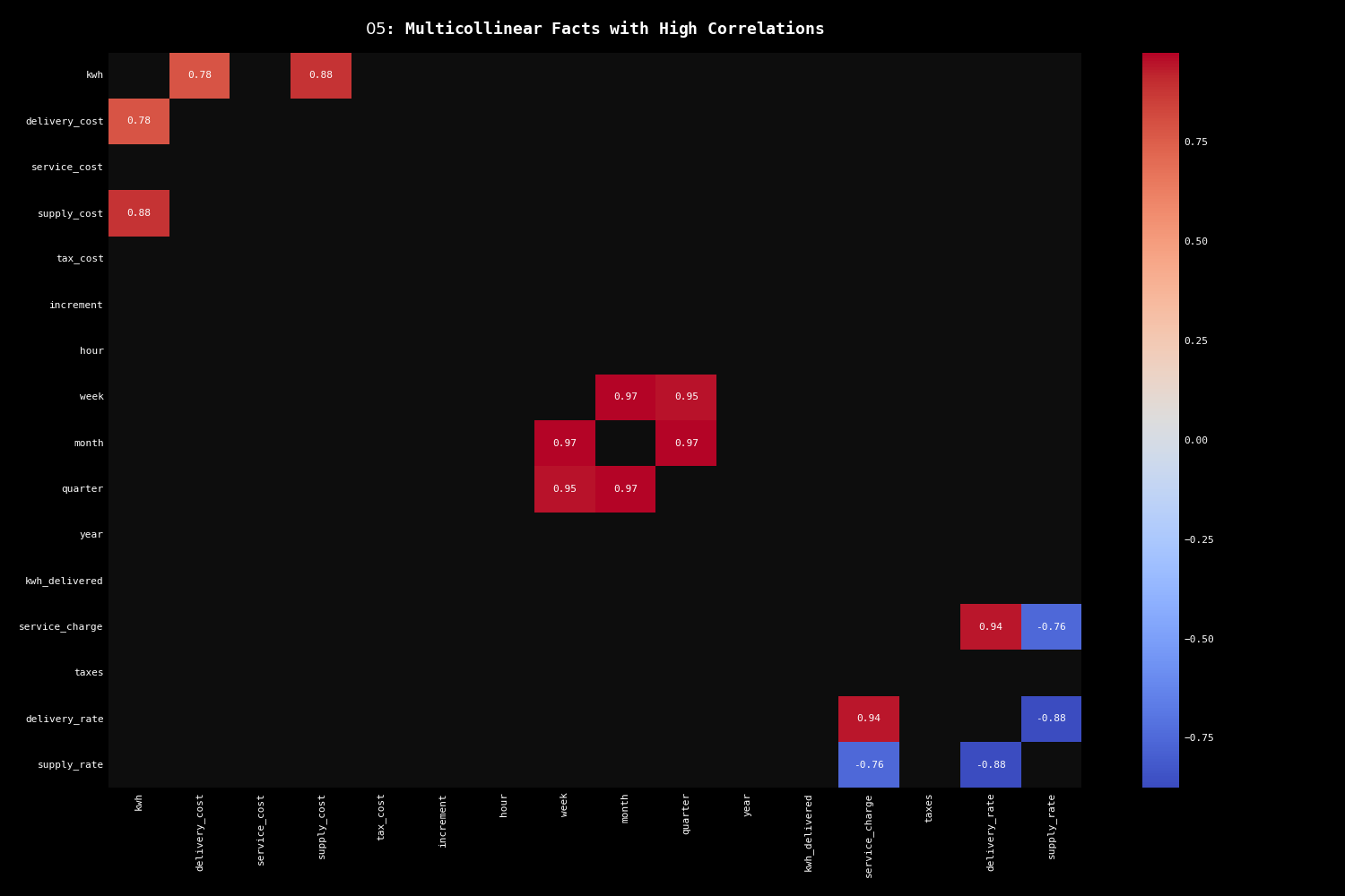
make jp05

Following the outlier removal, our next analytical step involves addressing multicollinearity among the features. This step is crucial in avoiding preconceived notions or biases from influencing the selection of numeric fields for our upcoming analyses. By systematically identifying highly correlated variables, we aim to let the data guide our insights, rather than making arbitrary choices that could skew our understanding.

The presence of multicollinearity in our dataset is not unexpected. In our model, cost components such as total_cost are calculated using a variety of other variables, like delivery_cost, supply_cost, and ratio-based allocations involving kwh. However, while these relationships are expected, they can pose challenges in predictive modeling. High multicollinearity can lead to unstable estimates of regression coefficients, making it difficult to ascertain the true effect of each independent variable on the dependent variable, which is total_cost in this case.

In that sense, addressing and removing multicollinear fields is not just about statistical accuracy, but rather ensuring that the insights we gain are reflective of the true drivers of energy costs.

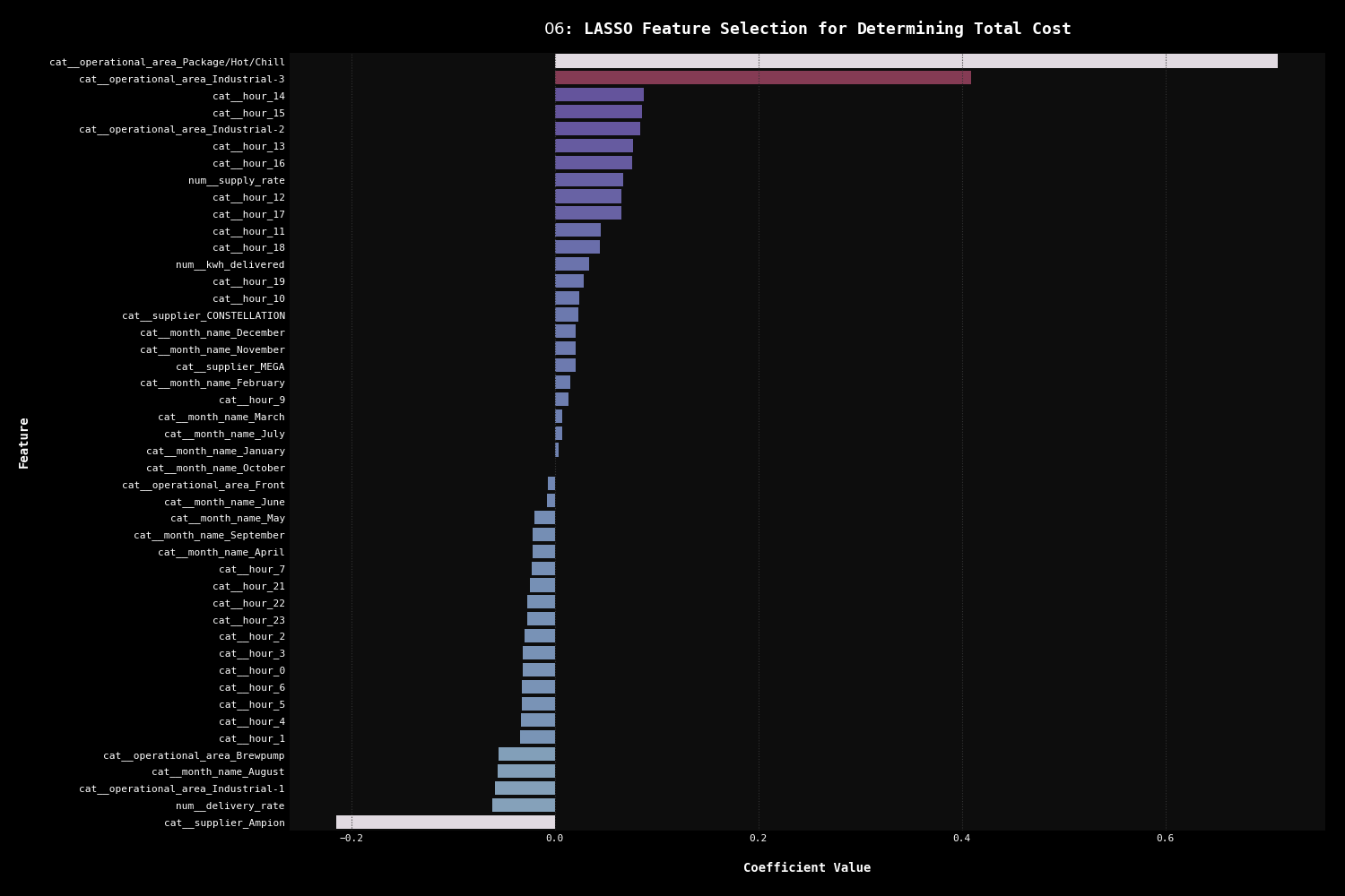
make jp06

With the dataset cleaned of anomalies and problematic fields, our primary objective is now to select the most relevant features from a broad range of possibilities, both categorical and numeric. Given the complex nature of our dataset, this selection process is crucial and must be approached with a method that is both unbiased and effective.

This is where LASSO (Least Absolute Shrinkage and Selection Operator) regression becomes an invaluable tool. LASSO is ideally suited for scenarios like ours, where the dataset contains a large number of potential predictors. It adeptly handles any missed multicollinearity and further simplifies the model by excluding less important features, making it more interpretable and manageable. Additionally, LASSO's regularization guards against overfitting, maintaining the model's effectiveness on both training data and new, unseen data.

The LASSO model has identified several key features, with operational areas related to heating, cooling, and industrial processes emerging as top predictors. These areas, particularly 'Package/Hot/Chill' and 'Industrial-3', underscore the significant impact of specific operational processes on overall energy costs. This finding aligns with our earlier analyses, emphasizing the critical role of these areas in driving energy expenditure, as they both generally increase over time in cost and usage.

Time-sensitive aspects of energy consumption are also highlighted in the model's output. Specific hours, particularly during the afternoon (from 12 PM to 5 PM), have been identified as influential, although the coefficients for each hour are modest. These hours typically coincide with increased production activities, heating or cooling demands, and other energy-intensive processes at the brewery. Therefore, the consistent importance of these afternoon hours in the LASSO model suggests that they are key periods where energy usage, and thus costs, are concentrated.

Furthermore, the model has revealed notable insights into the impact of different energy suppliers. Notably, the supplier 'Ampion', associated with solar energy, shows a significant negative coefficient, suggesting that opting for solar energy tends to lower total costs, in spite of our earlier analyses. The supplier 'CONSTELLATION' also emerges with a negative coefficient, implying cost savings when this supplier is chosen. In contrast, conventional suppliers like 'MEGA ENERGY' have positive coefficients, indicating a correlation with increased costs.

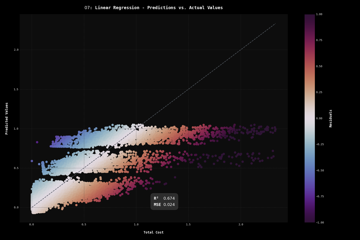
make jp07

We now have everything we need to start predictive modeling with Linear Regression, a logical step following our previous efforts in refining the dataset.

The Linear Regression model, applied to this curated dataset, achieved a Coefficient of Determination (R²) of 0.674 and a Mean Squared Error (MSE) of 0.024. These results indicate that the model successfully captures a substantial portion of the variance in the energy cost data. This R² value reflects the model's effectiveness in explaining the relationship between the selected features and energy costs, validating the relevance of the features identified by LASSO. However, the MSE, while relatively low, points to some prediction error, potentially due to complex, non-linear relationships in the data or other influential factors not captured by the current model.

The residual analysis, examining the differences between the actual and predicted values, shows a mean close to zero, indicating no significant bias in the model's predictions. However, the standard deviation of the residuals at 0.153 and the range of minimum and maximum residuals (from -0.775 to 1.666) highlight the presence of some large prediction errors. These suggest that specific scenarios or outliers are not fully captured by the model. The model's predictions also display a slightly narrower spread than the actual values, implying a conservative estimation in some cases.

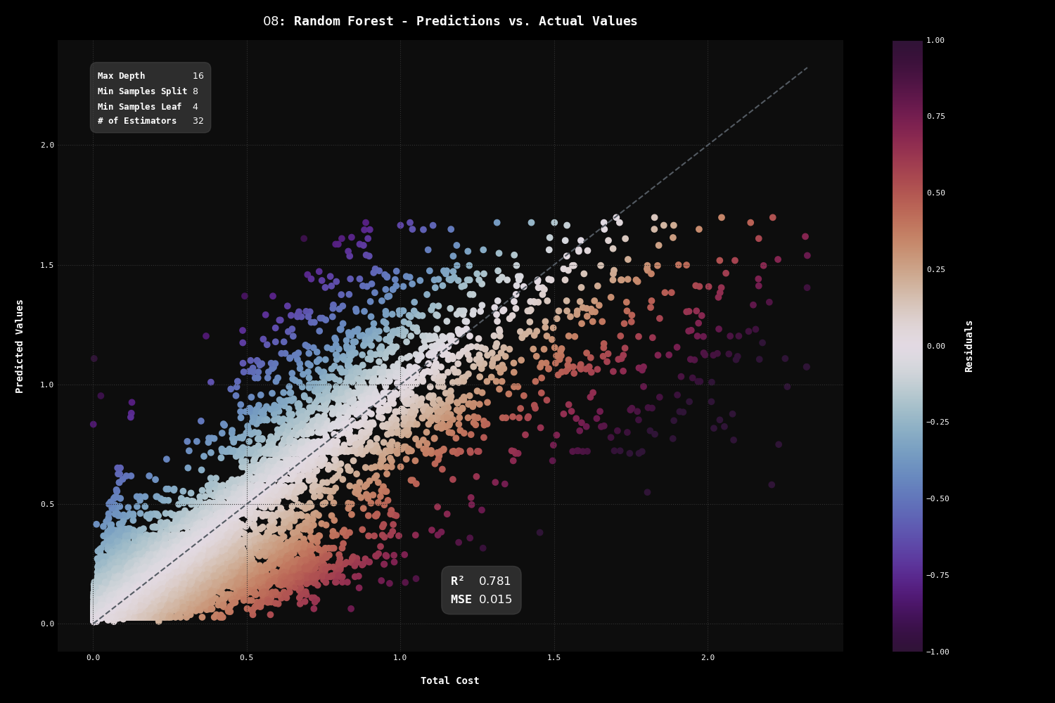
make jp08

Given the presence of prediction errors hinting at complexities beyond linear associations, we turned to a more sophisticated model capable of capturing intricate, potentially non-linear relationships within the data. For this, we chose Random Forest, an ensemble learning method known for its proficiency in handling complex datasets where linear models might struggle.

Our implementation of Random Forest demonstrated a notable improvement in predictive accuracy, achieving a Coefficient of Determination (R²) of 0.781 and a Mean Squared Error (MSE) of 0.015. These metrics indicate a significant enhancement in the model's ability to capture the variance in the brewery's energy costs compared to linear approaches. A lower MSE also demonstrates the model's increased accuracy in predictions, setting a robust foundation for our upcoming unsupervised recommendations.

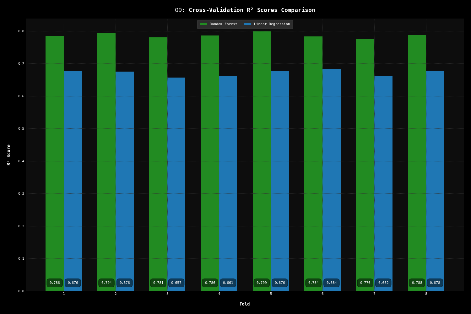
make jp09

From here, it is essential that we run cross-validation exercises on each of the models, as they provide a more robust and unbiased assessment of each model's performance. Cross-validation evaluates how well each model generalizes to an independent dataset.

In our cross-validation analysis, both models demonstrated similar performance consistency across different folds, as shown by their respective standard deviations in R² scores. The Random Forest model, with a standard deviation of 0.007, consistently achieved higher R² scores in each fold. This indicates its superior predictive ability compared to the Linear Regression model, which exhibited a slightly higher standard deviation of 0.009 and notably lower R² scores across the folds.

The decision to utilize more than the standard five folds (eight in this case) was intentional to rigorously test the models' integrity against random data splits. This approach strengthens our confidence in the models' performance, ensuring that the results are not skewed by specific data partitions.

make jp10

Having established a robust predictive framework through our analyses with LASSO and Random Forest, the next logical step is to bend this framework towards scenarios that align with the brewery's primary objective: maximizing kWh delivery while minimizing costs. This is where the strategic implementation of an optimization technique like SLSQP (Sequential Least Squares Quadratic Programming) becomes invaluable.

Optimization techniques like SLSQP are adept at navigating through intricate data terrains to seek out specific goals, in this case, cost-efficient operational scenarios. They provide the analytical finesse to adjust various influential factors identified by LASSO within the prediction realm of our Random Forest model. This approach allows us to move beyond mere prediction and understanding of the data, enabling us to actively explore 'what could be' scenarios that are not only feasible within the existing operational framework but are also beneficial to the brewery's bottom line. In this case, we ask the optimization algorithm to hold the kwh_delivered steady, while freely moving the other 40+ features to see where the target, total_cost, can possibly land.

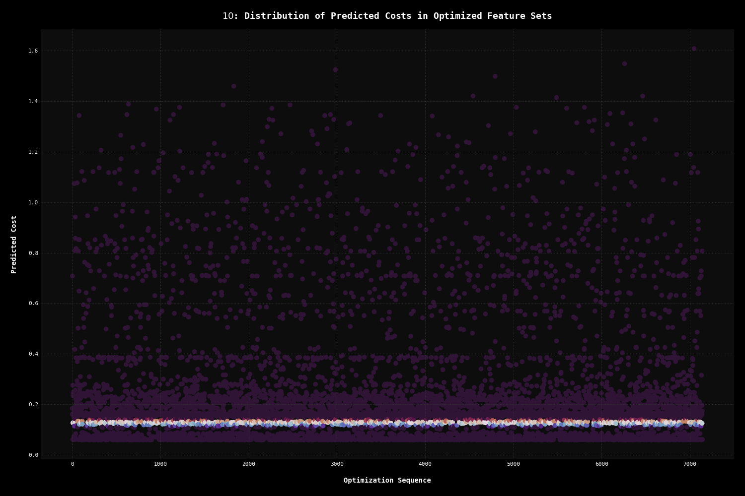
In executing this optimization, we set targeted cost bounds to an average of 75% of the mean total cost, creating a focused search area for the SLSQP algorithm. In doing so, we found 888 local minima (or possibilities) that fell within our desired cost efficiency range.

Of the other thousands of minima discovered, we see a broad range of predicted costs from our optimization, extending from exceedingly low to high, which demands careful scrutiny. While the lower end of this spectrum presents seemingly attractive cost figures, some of these scenarios might border on the ludicrous when translated into real-world operations. For example, an optimization result suggesting minimal operational hours to significantly reduce costs (effectively implying a shutdown) is trivial from a business standpoint.

By filtering out the extremes and focusing on the middle ground - scenarios that offer tangible cost reductions without compromising operational integrity - we ensure that the optimization process yields useful results.

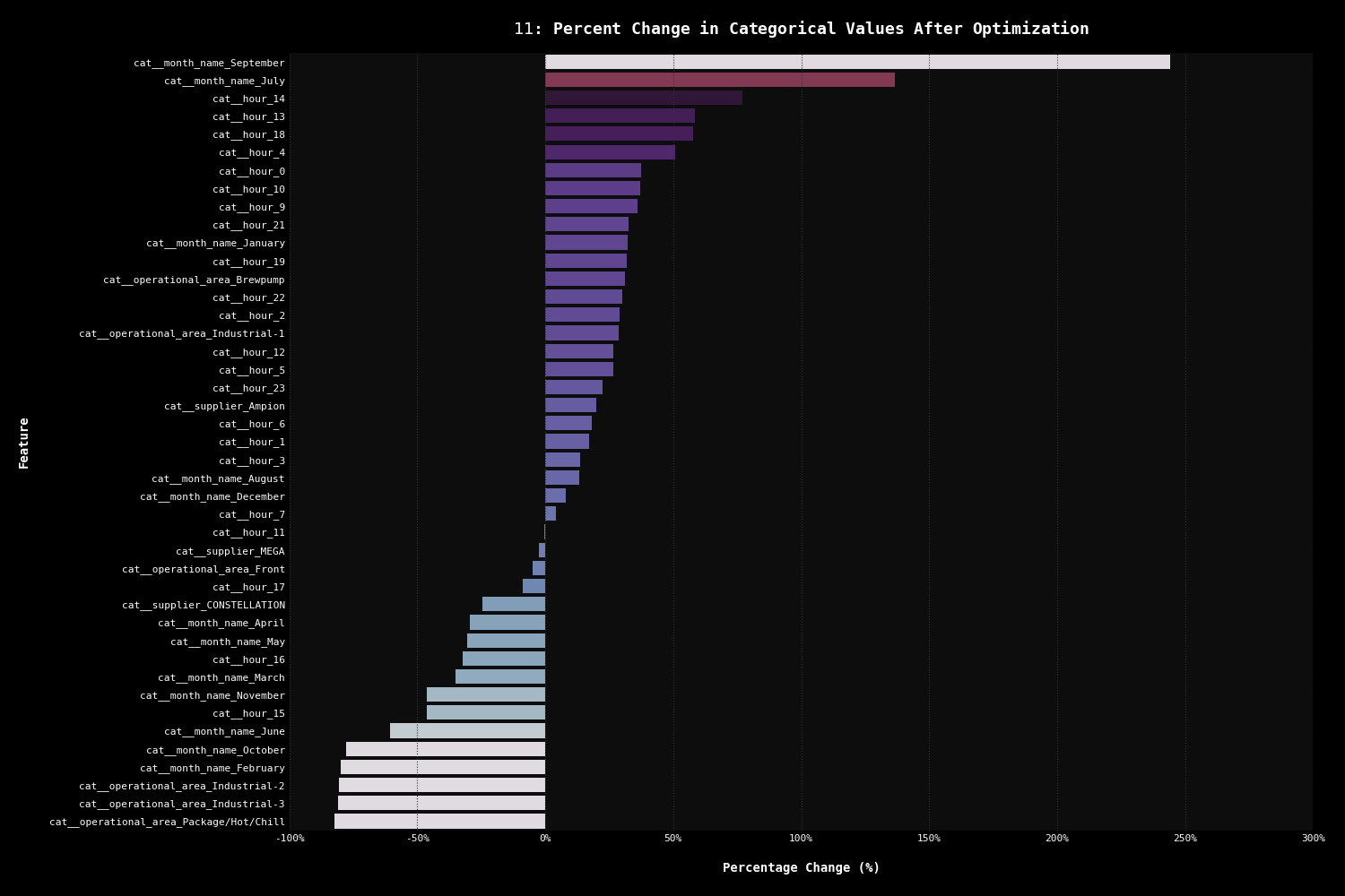
make jp11

For the concluding phase of our unsupervised analysis, we turn our attention to understanding the impact of our optimization efforts on various operational features picked by LASSO and amplified in predictive power by Random Forest.

Understanding the Final Metric

The percent changes we observe are a measure of how much more or less frequently (or intensely) a particular feature appears in the optimized scenarios compared to the original dataset. A positive percentage indicates an increase in the feature's influence in the optimized cost-efficient scenarios, while a negative percentage suggests a decrease.

These changes don't directly describe costs, but rather how each operational feature contributes to achieving the desired cost-efficiency.

Seasonal and Hourly Patterns

Summer Months and Early Hours: The significant increases in 'cat__month_name_September' (244%) and 'July' (137%) highlight the potential for strategic energy management in summer months, aligning with higher solar energy production balanced with cheaper conventional energy. Contrary to our initial focus on winter energy demands, this suggests summer months as pivotal for leveraging solar power, especially in Maine's climate. The emphasis on early hours like '4' (51%) and '0' (38%) could reflect operational strategies for tapping into conventional energy when it's most cost-efficienct, reinforcing the hypothesis that a shift in high-energy processes to these times could reap huge benefits.
Afternoon Operational Efficiency: The attention to afternoon hours 'cat__hour_14' (77%) and '13' (59%) aligns with our earlier observations of peak operational activities and high energy costs during these times. Rather than expanding operations, the brewery might benefit from optimizing existing processes in these hours.

Operational Areas: A Focus on Efficiency

Leveraging Consistent Usage Patterns: The analysis highlights 'cat__operational_area_Brewpump' (31%) and 'Industrial-1' (29%) as areas with consistent usage patterns, suggesting their operations are already streamlined and efficient. This consistency is beneficial, as it implies stable energy consumption without the inefficiencies associated with frequent system shutdowns and startups. In these areas, maintaining the current operational rhythm appears to be advantageous, allowing the brewery to leverage these stable patterns for ongoing energy efficiency.
Reassessing Areas with High Variability: In contrast, the large decrease in influence of 'Package/Hot/Chill' (-82%) and 'Industrial-3' (-81%) in the optimized scenarios suggests these areas have room for improvement in terms of energy efficiency. Unlike the consistently used areas, these might be experiencing variability in energy consumption, potentially due to irregular operation or less efficient equipment. Focusing on optimizing these areas, possibly through process improvements, upgrading to energy-efficient equipment, or reevaluating operational schedules, could lead to significant savings.

Supplier Selection and Energy Costs

Solar Energy's Balanced Role: The positive change in 'cat__supplier_Ampion' (20%) reflects a more nuanced role for solar energy than initially thought. Despite its higher costs, as observed in earlier analyses, this finding suggests Austin Street Brewery might consider a balanced approach, where solar power complements rather than fully replaces conventional energy sources, optimizing both costs and environmental impact based on availability of other power sources.
Supplier Dynamics in Cost Management: Changes in the influence of suppliers like 'MEGA' (-2%) and 'CONSTELLATION' (-25%) underscore the impact of supplier choice on energy cost management. Earlier findings highlighted the variability in costs with different suppliers. This optimization suggests exploring strategic supplier partnerships or negotiating favorable rates with suppliers like 'CONSTELLATION' to control operational costs effectively.

Major Takeaways

Solar is more expensive, but that said, you can bank credits in the summer and use them in the winter.
Heating and cooling dominate the cost profile for the company, and should be a focus for cost optimization.
Because energy usage is greatest during peak hours, a shift to a variable rate (Mid/On/Off Peak) would be more costly.
The structure of the data lends itself well to prediction and an opportunity to revisit as the business changes.

Acknowledgments

This project was shaped under the supervision of Professor Philip Bogden during our Intro to Data Management class at the Roux Institute of Northeastern University.

We would like to express our gratitude to Professor Bogden for his consistent guidance and invaluable insights. Our thanks also extend to our TA, Meghana Chillara, for her patience, consistently timely input, and collaboration with each of us. Special thanks to both Harsh Bhojwani and Anurag Daga as well, for helping us keep our spirits high and reminding us to take a step back at the most impactful times.

jparkington / Electric-Brew