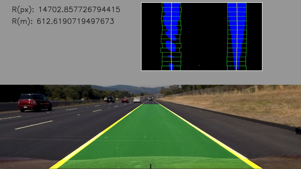
Advanced Lane Finding Project
Python project to explore the topic of advanced lane finding. This project is created as one possible solution to the second project of Udacity's Nano Degree Self Driving Car Engineer in the School of Autonomous Systems.
Goal
The goals / steps of this project are the following:
- Compute the camera calibration matrix and distortion coefficients given a set of chessboard images.
- Apply a distortion correction to raw images.
- Use color transforms, gradients, etc., to create a thresholded binary image.
- Apply a perspective transform to rectify binary image ("birds-eye view").
- Detect lane pixels and fit to find the lane boundary.
- Determine the curvature of the lane and vehicle position with respect to center.
- Warp the detected lane boundaries back onto the original image.
- Output visual display of the lane boundaries and numerical estimation of lane curvature and vehicle position.
A full project rubrick can be found from the project specification (when logged in to Udacity).
Setup
This work has been created with the help of Docker in order to keep your local environment clean and for easy execution of the pipeline. When Docker is installed, running make run from the repo root directory will start the Docker container and run the pipeline. Output from the pipeline will end up into the assets/output_images directory.
The images for camera calibration are stored in the folder called assets/camera_cal.
The images in assets/test_images are for testing the pipeline on single frames.
Read more about the setup
1. Camera Calibration
The code for this step is contained in the class DistortionCorrector found in alf/pipeline/distortion_corrector.py.
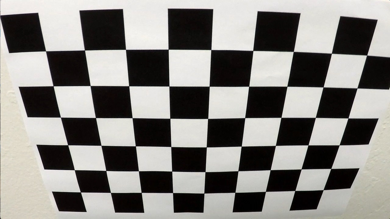
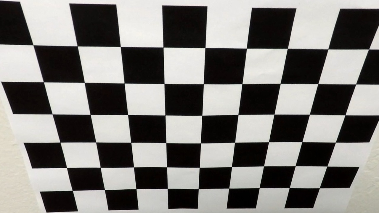
Before using the DistortionCorrector it needs to be calibrated by passing a set of images to its calibrate method. For each valid calibration image, its corners are found and stored to a collection. At the same time a collection is updated with the point indexes.
Once all the calibration data is collected, an image can be undistorted by using the undistort method form the same DistortionCorrector object. An example is shown in the table below:
| Input | Output |
|---|---|
 |
 |
2. Pipeline (single images)
2.1 Distortion correction
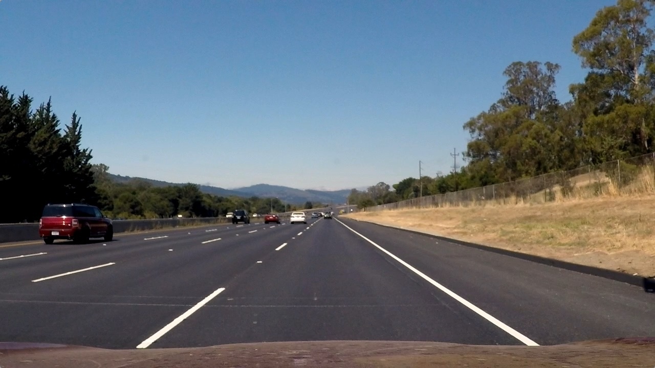
Once we have a calibrated DistortionCorrector object as described in section 1.1. we can simply apply the undistort method on any of our test images found from the ./assets/test_images directory. The effect can be seen from the table below.
| Input | Output |
|---|---|
 |
 |
As the calibration step can take some time, we should make sure the DistortionCorrector is calibrated only once during the pipeline processing.
2.2 Binary Threshold
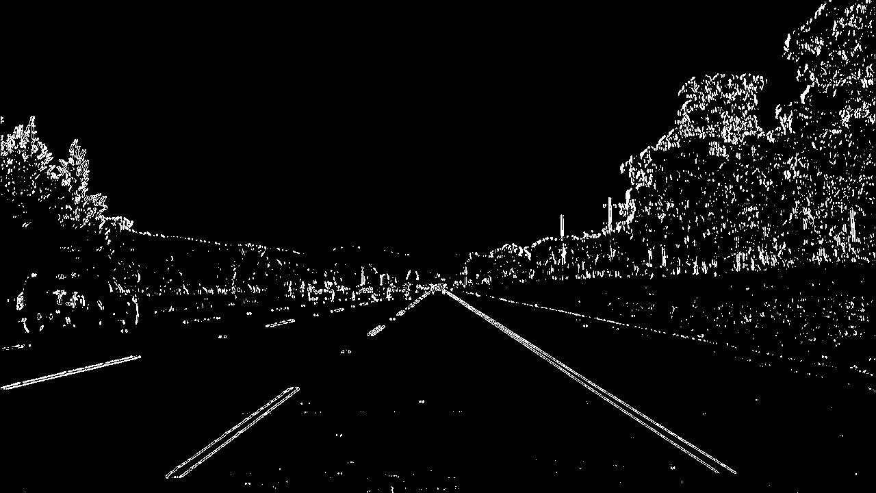
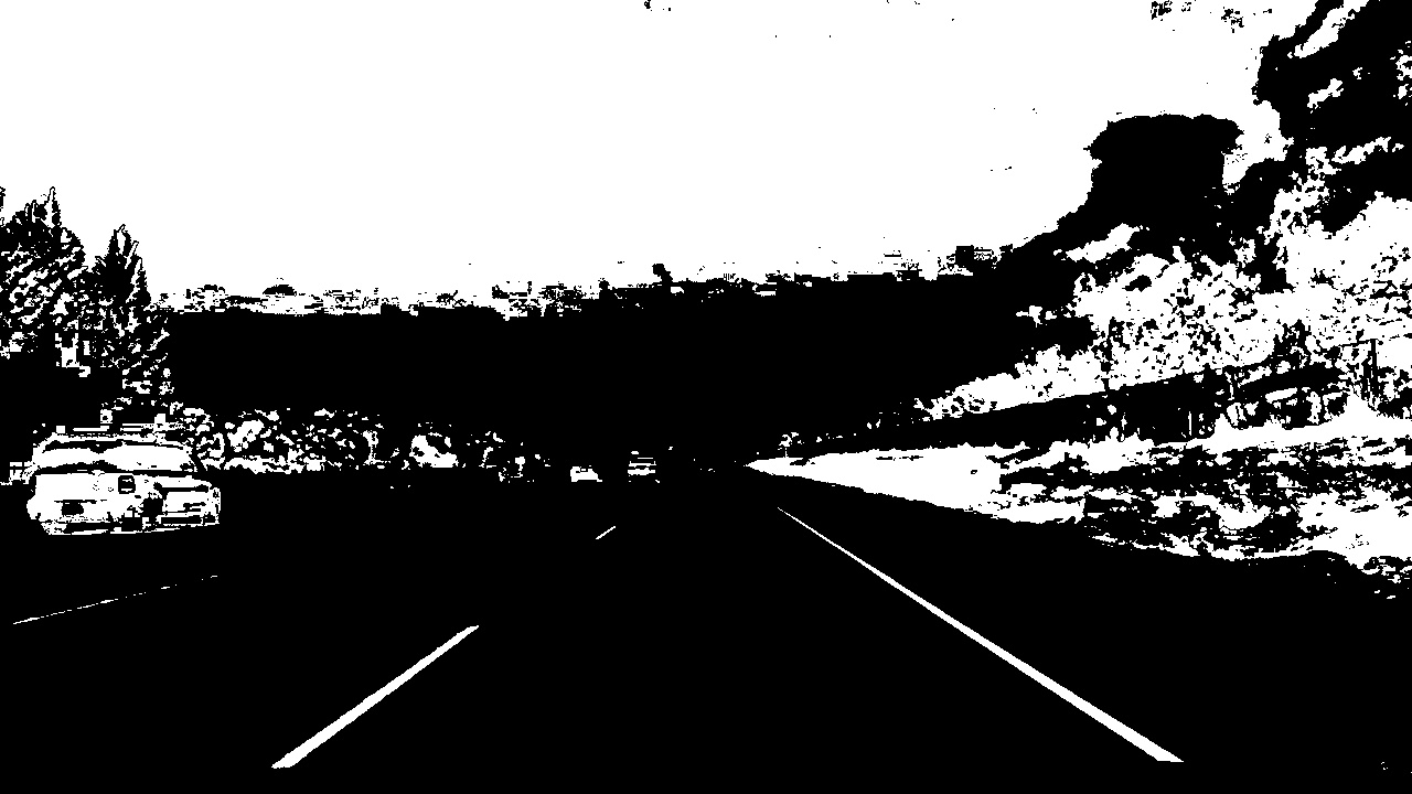
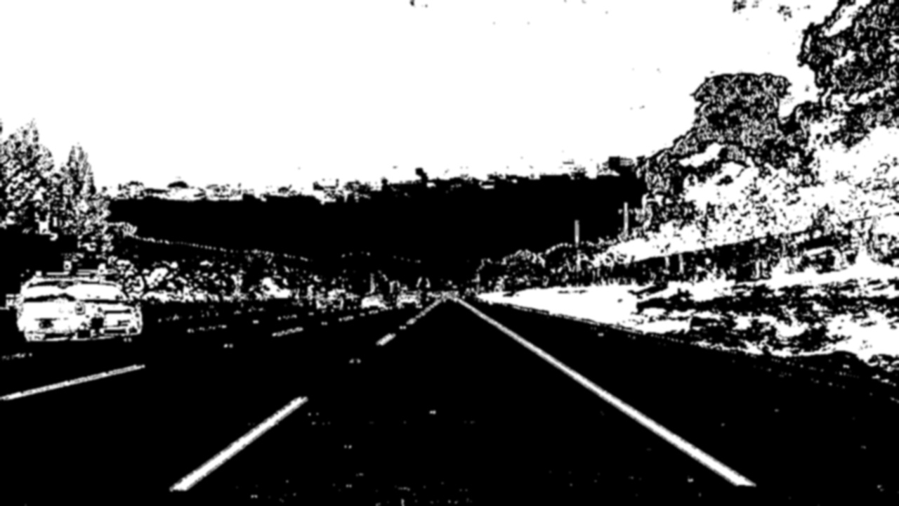
With a ImageThresholder object, created from its class found in ./src/alf/pipeline/thresholder.py, both color and gradient thresholds are applied to an image in the threshold() function. This function combines the threshold results as a binary image. The table below shows input, gradient thresholded, color thresholded and both threshold combined.
| Input | gradient threshold |
|---|---|
 |
 |
| color threshold | combined thresholds |
|---|---|
 |
 |
2.3 Perspective Transform
The perspective transform requires the knowledge of a set of source points which then are mapped onto desired destination points. We will find them manually for now but trying to find both sets automatically seems a good usecase for reusing code from lane finding project.
The source and destination points are created in the Roi class found in alf/common/roi.py.
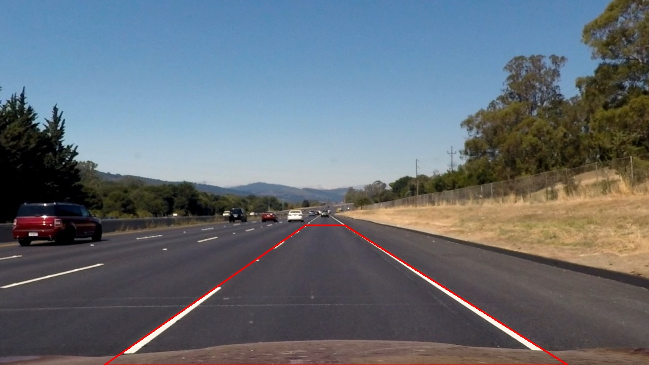
For the source points I chose values that created a snug fit on the outsides of the lane when plotted on the .assets/test_images/straight_lines2 image. The desination points are based on the source points whereby the upper point position are changed so that the resulting polygon becomes a square. This resulted in the following source and destination points:
| SRC points | DST points |
|---|---|
| 602, 444 | 305, 0 |
| 680, 444 | 1020, 0 |
| 1120, 720 | 1020, 720 |
| 205, 720 | 305, 720 |
I verified that my perspective transform was working as expected by drawing the src points onto a test image and then inspect that the perspective transformed counterpart contained the points in a rectangular fashion.
| Input | Source points (marked) | Warped (marked) |
|---|---|---|
 |
 |
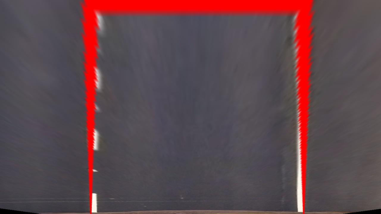 |
The images contain the points and lines for illustrative purposed, they will not be drawn in the actual pipeline. It seems that the transform is succesful as the bounding box is a rectangle and the lane lines can be considered to be perpendicular to each other as in the original picture.
2.4. Polynomial fitting of lane lines
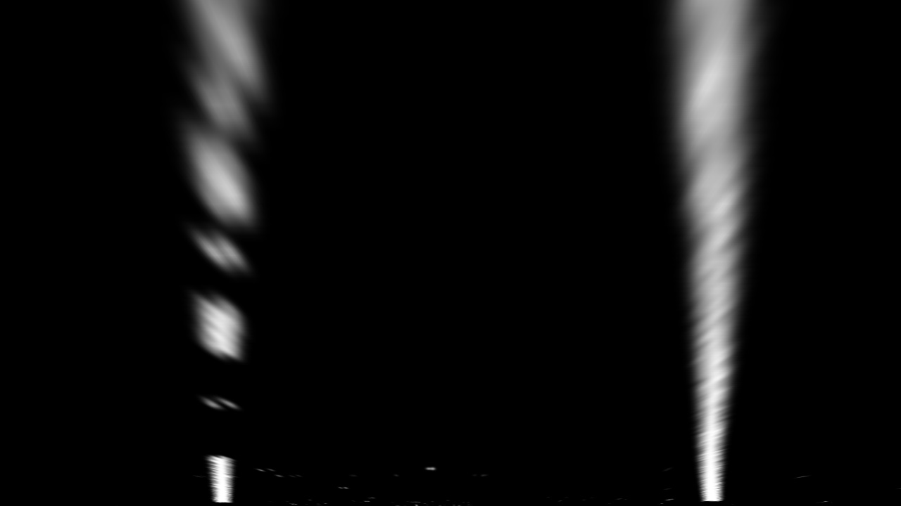
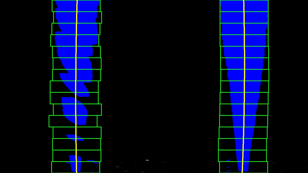
First, from the perspective transformed binary lane frame the line x positions are found with the help a histogram. Then an amount of sliding windows (green) are placed iteratively over the lane pixels from bottom to top. The pixel indices (x and y values) are then used to fit a polynomial (yellow).
| Input | Windowed Search |
|---|---|
 |
 |
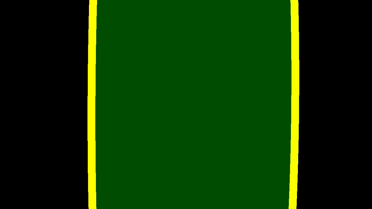
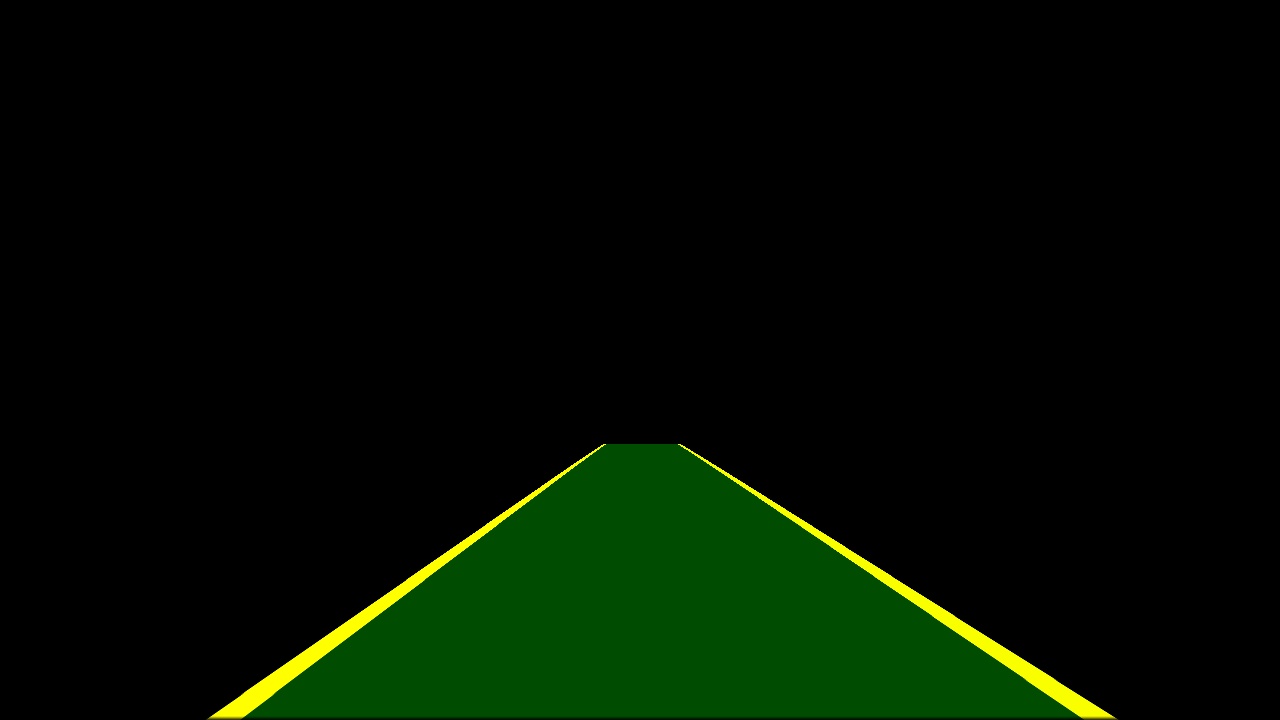
From the data found the left and right lines are drawn and the lane itself is filled. This visualisation is then perspective transformed back into the original frame perspective.
| Lane visualisation | Original perspective |
|---|---|
 |
 |
2.5. Radius of curvature of the lane and vehicle position with respect to center
-- TBD
2.6. Lane area visualization
The lane visualisation is taken care of within the alf/processor.py file.
A copy of the perspective transformed lanes with polylines and windows is resized and placed within the
end result of the pipeline.
3. Pipeline (video)
Here's a link to my video result
Discussion
The current pipeline works good enough for the first video, it is stable enough during the whole lenght. Due to the lane length chosen the upper bounds of the lines are not detected in a precise manner as they move out of their measured pixel space (left vs right halves of frame).
Improvements such as masking, keeping a running average and use that when data is missing from a few sequential frames would improve the algorithm.
