
Building off the first lane finding project, this project attempts to build a more robust system for detecting lane markings with a front-facing camera.
We were able to detect lane markings for two simple scenarios. The steps to determine the line markings were; first, we preprocess the image using a combination of Sobel filters and different color spaces. This will isolate the line markings within the image. Second, We transform those image into a top-down view and use a sliding histogram window to arrive at a point cloud of potential line matches. Then we then fit a curve to those lines and reproject the lines back into the driving space. Finally, we apply a simple Kalman filter to reduce the impact of errors and smooth out the curves
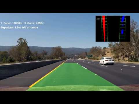
The above video shows the detection algorithm in progress (in green). In the top right corner we can see the intermediary images used to locate the lane markings. Road curvature and offsets are derived as a part of the detection algorithm.
-
environment.ymlis the Anaconda dependencies for the project.conda env create -f environment & source activate AdvLaneFindingshould prepare the environment -
Run the video processor
usage: video_processor.py [-h] -i INPUT -o OUTPUT [-c CAMERA]

optional arguments:
  -h, --help            show this help message and exit
  -i INPUT, --input INPUT
                        Input video file
  -o OUTPUT, --output OUTPUT
                        Output video file
  -c CAMERA             Calibration File from calibrate.py
1. Compute the camera calibration matrix and distortion coefficients given a set of chessboard images, and Apply a distortion correction to raw images.

Using the provided images within the camera_cal directory, a correction file was created to adjust images for camera distortion. The program is run with.
python calibrate.py [image_directory]This generates a camera.p pickle file which will be used in the remaining goals.
The calibration is done with the following steps;
- All the images in the directory and loaded and converted to gray scale. One image is removed from the set to be used for verification testing.
- Since we are using a regularly spaced grid we can calculate the destination grid coordinates.
- OpenCV provides a method to calculate the source coordinates with
cv2.findChessboardCorners - Mapping those source to the destination provides a transform matrix and that matrix is stored in the pickle file for retrieval
- The isolated image is then reprojected using the transform matrix to visually verify the results.(See image above)
The next 4 steps involved transforming the images into a format that will help to determine the line markings. To this end the program image_processing_test.py was created to demonstrate a processing pipeline with still images used to optimize the algorithms.
python image_processing_test.py [input image] -c camera file(optional) -o output image (optional)
The output of that program is an image file (below), containing all the intermediary images generated in creating the image processing pipeline.
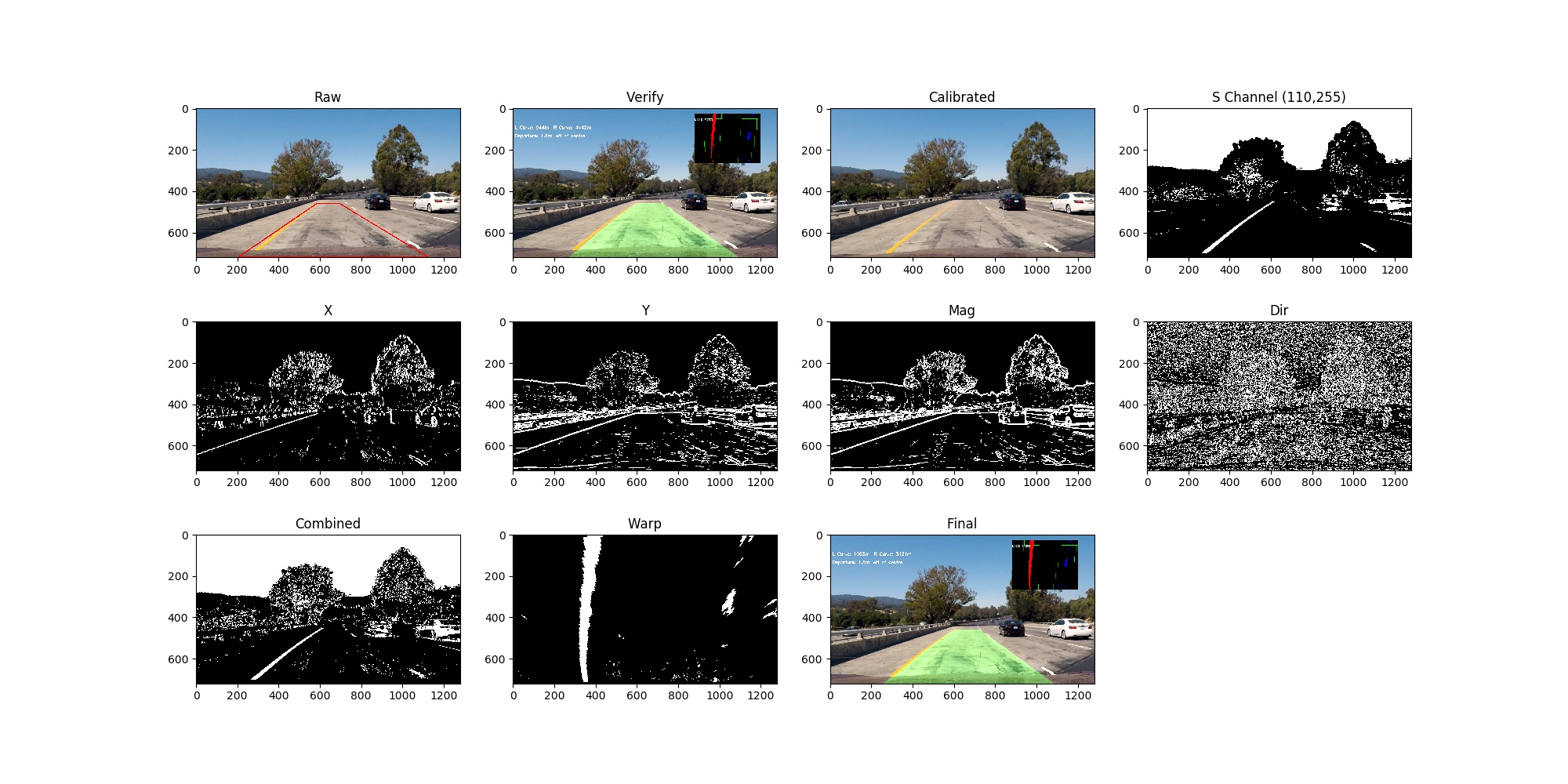
Here are the description of the images included;
| Image Name | Details |
|---|---|
| Raw | Raw Image, with perspective area highlighted |
| Verify | Check image to ensure the image processing is the sames as video processing |
| Calibrated | Raw Image after camera calibration applied |
| S Channel | Binary image is converted to HSL and the Saturation channel is extracted. |
| X | Sobel Filter only X direction |
| Y | Sobel Filter only Y direction |
| Magnitude | Magnitude of the Sobel Filter |
| Dir | Direction of the Sobel Filter |
| Combined | The merged image from the pipeline (see below) |
| Warp | The combined image with the perspective warp applied |
| Clipped | 100 pixels from the left and right side of the warp image |
| Histogram | Visualization tools for the histogram search |
| Final | Post histogram determination and mapped into driving space |
In this step we hope to highlight the lane markings in the image and remove the noise from external influences. To do this we implement a combination of the image processing algorithms above. After much trial-and-error we arrived at a solution for our current video.
The combined image was those pixels that passed either;
- Saturation Filter between pixel values of 110 and 255, or
- Sobel Direction between 0.1 and 1.1 (pi) and Sobel Magnitude greater than 30
Trial-and-error was used to determine the filter combination and I suspect a more rigorous approach should be used. The types of filters had a very large impact on the results and would vary between different driving conditions. This combination was chosen to work well with the given test data.
Full Size Images Test 1 Test 2 Test 3 Test 4 Test 5 Test 6 Test 7 Test 8
After processing the images to highlight the lines, the next step is to transform the image from a driving perspective to a top-down view. This simplifies much of the calculations for lane determination. By using some knowledge of the location of the front facing camera we can estimate the road in driving perspective. The "Raw" image (above) shows the perspective in red that is to be transformed into a top down reference.
Once we have the perspective, we can transform the image using cv2.getPerspectiveTransform(src, dst). The "Combined" image and the "Warp" image show how the transformation occurs.
Transform parameters
    img_size = (img.shape[1], img.shape[0])
    src = np.float32(
        [[(img_size[0] / 2) - 55, img_size[1] / 2 + 100],
        [((img_size[0] / 6) - 10), img_size[1]],
        [(img_size[0] * 5 / 6) + 60, img_size[1]],
        [(img_size[0] / 2 + 55), img_size[1] / 2 + 100]])
    dst = np.float32(
        [[(img_size[0] / 4), 0],
        [(img_size[0] / 4), img_size[1]],
        [(img_size[0] * 3 / 4), img_size[1]],
[(img_size[0] * 3 / 4), 0]])Once the image has been mapped into top-down we can select points that mark the lane by choosing the pixels on the left or right side and performing a curve fit on those pixels. Given that not all of the pixels are associated with either lane marking we need to be particular about selecting the correct points. To do this we create a buffer of around 100 pixels around the predicted area where the lane markings should be. But this requires prior knowledge of the lane line. (In practical terms we create the buffer using a series of sliding rectangles to speed the calculations.)
But this requires a-priori knowledge of where the lane markings should be. We can gather this information in one of two ways;
- If there is no previous lane marking information; With no reference information we assume the location of the left and right lanes will correspond with the largest density of points. By taking a histogram of the bottom half of the image we can find the left and right starting points as the peaks of that histogram. Since we only need to seed the buffer, the accuracy requirements are low. We can then use that starting reference and tile windows above it shifting it left or right based on the density of the pixels in the new window.
Histogram Section within ImageProcessor.py
- If we have previous reference lane geometry; We use the lane geometry as a centerline reference for the search windows and create a buffer around the lane in that manner.
The "Histogram" images above and the floating window in the demonstration video illustrate how the system works. The white rectangles are the sliding window and the left (red) and right (blue) pixels are the point cloud. The reference video does an excellent job of visualizing the process in action.
Within the buffer we get a point cloud. From that cloud of points we can perform a simple least-squares polynomial curve fit. That curve represents a likely solution for the lane geometry.
The solution above requires information from previous epochs to improve the fit. But with any estimation, errors will propagate through a system and could cause the system to fail. In our model we employ a simple Kalman filter to maintain both the current state and provide an estimate of the accuracy of the solution. Using both the filter and some sanity checks we can provide a system that both smooths the results and provides an estimate of the accuracy of the solution.
The Kalman filter uses the parameters (A,B,C) from the polyfit calculation as measurements, and the polyfit covariance error as the accuracy estimate of the solution. The model uses a random walk process so it runs the same as a weighted average over multiple epochs. After each epoch we evaluate the results against the sanity checks to make sure they match with our expectations. If not, we reset the filter and start the search over again.
measurement = [A B C]
P = [Pa Pb Pc] # From np.polyfit(...cov=True...)
# H=Q=F are identity matrices

# UPDATE x, P based on measurement m
# distance between measured and current position-belief
y = np.matrix(measurement).T - H * x
S = H * P * H.T + R  # residual convariance
K = P * H.T * S.I    # Kalman gain
x = x + K*y
I = np.matrix(np.eye(F.shape[0])) # identity matrix
P = (I - K*H)*P

# PREDICT x, P based on motion
x = F*x + motion
P = F*P*F.T + Q
The sanity checks look for;
- Parallelism. The two lane curves should be roughly parallel in the top-down space. We can compare the A, B terms of the curve fit and hold them to a small threshold. If the threshold is exceeded we can be confident our solution is not correct.
- Residual Errors. The Kalman filter produces an estimate for each epoch and compares it to the measurements. If those two numbers are vastly different either the model is wrong or the lane calculation is wrong. Resetting the filter allows the two to sync back together
Once the two lane geometries were estimated we calculate some terms around the curvature and the offset from center (assuming the camera is in the middle of the vehicle).
The curvature is determined with;
    # Line.py
    # Define conversions in x and y from pixels space to meters
    ym_per_pix = 30/720 # meters per pixel in y dimension
    xm_per_pix = 3.7/700 # meters per pixel in x dimension

    y = np.array(np.linspace(0, 719, num=10))
    x = np.array([fit_cr(x) for x in y])
    y_eval = np.max(y)

    fit_cr = np.polyfit(y * ym_per_pix, x * xm_per_pix, 2)
    curverad = ((1 + (2 * fit_cr[0] * y_eval / 2. + fit_cr[1]) ** 2) ** 1.5) / np.absolute(2 * fit_cr[0])
The offset is taken by averaging the two lane geometries to arrive at a center geometry. From that geometry we calculate where it intersects the bottom of the image and compare that to the center of the image. The distance in pixels is then converted to meters.
    # ImageProcessor.py
    center_poly = (left_line.get_as_poly() + right_line.get_as_poly()) / 2
offset = (720 / 2 - center_poly(719)) * 3.7 / 700Finally, we take the predicted lane geometries and draw them on a blank image. We then apply the warping method in reverse to translate that image back to drive perspective. We overlay that image on the original image to show visually where the solution matches.
For the final output we also include, left and right curvatures, offsets and the picture window showing the top-down calculations.
This lane determination project had a slightly different approach than earlier projects. Instead of trying to determine the markings epoch by epoch, I wanted to use a Kalman filter to create an internal state and use the marking information to improve that state where possible. This allowed the system a much more flexible way to handle the data and we were less effected by outliers and bad measurements.
In processing the videos, I ran into a some issues;
-
Parallel markings or barriers One issue that was seen in the video was that the presence of a concrete road barrier parallel to the road markings that can often be confused as a lane marking. We compensate by doing a clipping process on the leftmost and rightmost pixels in the image. This eliminates some of the outliers on the edges of the image and enables the histogram to work slightly better
-
Different lighting conditions The fixed set of filters responded differently based upon the lighting in the image, either shadows or changes in the road colors. This resulted in wildly incorrect lane calculations. Inside the Kalman filter we compensate by reducing the impact of uncertain solutions in our state. In some cases the measurements were discarded entirely.
-
Rapid road swerves In the harder_challenge.mp4 video, the course was a swerving road at slow speed with many turns. In this case both the algorithm for lane detection and the Kalman filter were not able to keep up. For the image filtering; we were not able to calculate quick turns because of the thresholds set in the image processing. Increasing the threshold causes too much of the image to pass through causing incorrect curve fit solutions. The Kalman filter didn't have a sufficient internal model to handle multiple curves within a single image. There was some work on fitting a cubic or higher spline to the road geometry, but without accurate road measurements from the images it would not be possible to guage their accuracy. More work would be needed to be done to determine how best to process images from this video to locate the markings.
-
Non-parallel lane markings While I didn't run into this case in the videos, there are plenty of scenarios where the markings may be missing on either side. This algorithm will do everything possible to locate the markings. In the event they are missing, the algorithm extrapolates from previous measurements. This prediction can handle short gaps well enough. I purposefully removed filters on lane size, and calculate the left and right independently. This should work well enough to handle this case.
The two optional video files performed moderately well (challenge.mp4) and poorly (harder_challenge.mp4) with the same algorithm. This indicates that solution may not be suitable for all cases. Some of the issues that could help out the algorithms are;
Image Preprocessing The algorithm is dependent upon reasonably accurate estimates for lane markings. Issues such as changes in lighting, road textures, or parallel road barriers would often show up as errors within the data which were very difficult to filter out. Changing the parameters of the image filters and combinations worked in some situations but not others. There didn't seem to be a generic model to handle those cases. It might be worth some research time to apply either multiple filtered images in parallel or a deep-learning algorithm to change the filters dynamically. Both would help out immensely
Kalman Filtering The Kalman filter algorithm proved to be an excellent tool within this project. The single algorithm was able to predict outliers, smooth rough data and provide a very accurate interpolation estimate when results were not available. But the implementation that I created used the most basic of assumptions. It can be easily modified to;
- Apply a single filter to match both right and left lines with a constraint they should be roughly parallel,
- Apply a transition matrix that takes into consideration how the lanes are expected to change based on the actual road construction information
- Use the filter with mapping data to provide a better estimate on the curvature.
Any of those changes would make for a much better solution and would be well suited for even the most complex of road conditions.
Error Modeling I tried multiple approaches to modeling the errors in the system. With good error estimates we can control outliers and maintain a better estimate on the system. The best error estimate I arrived at was using the least-squares errors from the polyfit algorithm. This gives me the error in fitting the line which isn't always correlated to the ground truth accuracy.