![]()
This pangenome graph construction pipeline renders a collection of sequences into a pangenome graph (in the variation graph model). Its goal is to build a graph that is locally directed and acyclic while preserving large-scale variation. Maintaining local linearity is important for the interpretation, visualization, and reuse of pangenome variation graphs.
It uses three phases:
-
wfmash: (alignment) --
wfmashuses a modified version of mashmap to obtain approximate mappings, and then applies a wavefront-guided global alignment algorithm for long sequences to derive an alignment for each mapping.wfmashuses the wavefront alignment algorithm for base-level alignment. This mapper is used to scaffold the pangenome, using genome segments of a given length with a specified maximum level of sequence divergence. All segments in the input are mapped to all others. This step yields alignments represented in the PAF output format, with cigars describing their base-exact alignment. -
seqwish: (graph induction) -- The pangenome graph is induced from the alignments. The induction process implicitly builds the alignment graph in a memory-efficient disk-backed implicit interval tree. It then computes the transitive closure of the bases in the input sequences through the alignments. By tracing the paths of the input sequences through the graph, it produces a variation graph, which it emits in the restricted subset of GFAv1 format used by variation-graph-based tools.
-
smoothxg: (normalization) -- The graph is then sorted with a form of multi-dimensional scaling in 1D, groomed, and topologically ordered locally. The 1D order is then broken into "blocks" which are "smoothed" using the partial order alignment (POA) algorithm implemented in abPOA or spoa. This normalizes their mutual alignment and removes artifacts resulting from transitive ambiguities in the pairwise alignments. It ensures that the graph always has local partial order, which is essential for many applications and matches our prior expectations about small-scale variation in genomes. This step yields a rebuilt graph, a consensus subgraph, and a whole genome alignment in MAF format.
Optional post-processing steps provide 1D and 2D diagnostic visualizations of the graph, basic graph metrics.
The output graph (*.smooth.gfa) is suitable as input to vg deconstruct to obtain a VCF file relative to any set of reference sequences used in the construction, or for read mapping in vg or with GraphAligner.
pggb requires at least an input sequence -i, a segment length -s, and a mapping identity minimum -p.
Other parameters may help in specific instances to shape the alignment set.
Using a test from the data/HLA directory in this repo:
git clone --recursive https://github.com/pangenome/pggb
cd pggb
./pggb -i data/HLA/DRB1-3123.fa.gz -N -w 50000 -s 5000 -I 0 -p 80 -n 10 -k 8 -t 16 -v -L -o out
This yields a variation graph in GFA format, a multiple sequence alignment in MAF format, a series of consensus graphs at different levels of variant resolution, and several diagnostic images (all in the directory out/).
By default, the outputs are named according to the input file and the construction parameters.
Adding -v and -L render 1D and 2D diagnostic images of the graph.
(These are not enabled by default because they sometimes require manual configuration. Additionally, 2D layout via -L can take a while.)
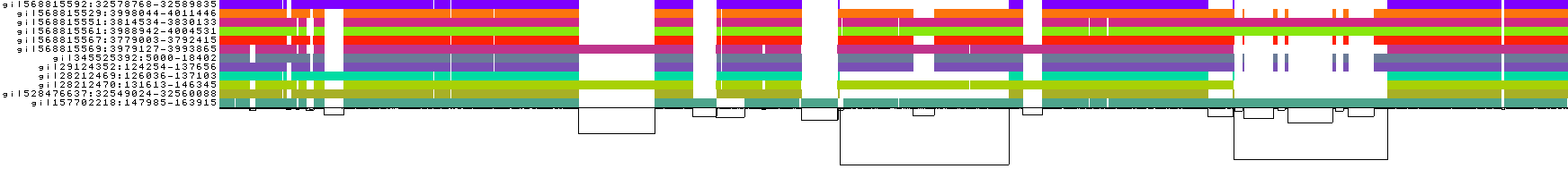
- The graph nodes’ are arranged from left to right forming the pangenome’s sequence.
- The colored bars represent the binned, linearized renderings of the embedded paths versus this pangenome sequence in a binary matrix.
- The black lines under the paths, so called links, represent the topology of the graph.
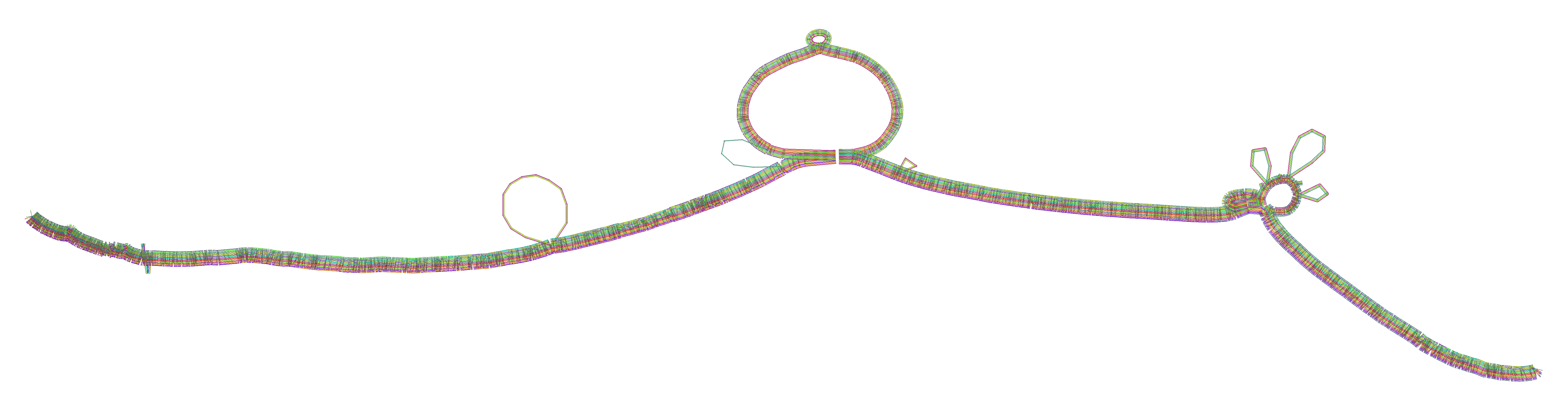
- Each colored rectangle represents a node of a path. The node’s x-coordinates are on the x-axis and the y-coordinates are on the y-axis, respectively.
- A bubble indicates that here some paths have a diverging sequence or it can represent a repeat region.
Although it makes for a nice example, the settings for this small, highly-diverse gene in the human HLA are typically too sensitive for application to whole genomes.
In practice, we usually need to set -s much higher, up to 50000 or 100000 depending on context, to ensure that the resulting graphs maintain a structure reflective of the underlying homology of large regions of the genome, and not spurious matches caused by small repeats.
To ensure that we only get high-quality alignments, we might need to set -p higher, near the expected pairwise diversity of the sequences we're using (including structural variants in the diversity metric).
In general, increasing -s, and -p decreases runtime and memory usage.
For instance, a good setting for 10-20 genomes from the same species, with diversity from 1-5% would be -s 100000 -p 90 -n 10.
However, if we wanted to include genomes from another species with higher divergence (say 20%), we might use -s 100000 -p 70 -n 10.
The exact configuration depends on the application, and testing must be used to determine what is appropriate for a given study.
To simplify installation and versioning, we have an automated GitHub action that pushes the current docker build to the GitHub registry. To use it, first pull the actual image:
docker pull ghcr.io/pangenome/pggb:latestOr if you want to pull a specific snapshot from https://github.com/orgs/pangenome/packages/container/package/pggb:
docker pull ghcr.io/pangenome/pggb:TAGGoing in the pggb directory
git clone --recursive https://github.com/pangenome/pggb.git
cd pggb
you can run the container using the example human leukocyte antigen (HLA) data provided in this repo:
docker run -it -v ${PWD}/data/:/data ghcr.io/pangenome/pggb:latest "pggb -i /data/HLA/DRB1-3123.fa.gz -N -w 50000 -s 5000 -I 0 -p 80 -n 10 -k 8 -t 2 -v -L -o /data/out -m"The -v argument of docker run always expects a full path: If you intended to pass a host directory, use absolute path. This is taken care of by using ${PWD}.
If you want to experiment around, you can build a docker image locally using the Dockerfile:
docker build --target binary -t ${USER}/pggb:latest .Staying in the pggb directory, we can run pggb with the locally build image:
docker run -it -v ${PWD}/data/:/data ${USER}/pggb "pggb -i /data/HLA/DRB1-3123.fa.gz -N -w 50000 -s 5000 -I 0 -p 80 -n 10 -k 8 -t 2 -v -L -o /data/out -m"abPOA of pggb uses SIMD instructions which require AVX. The currently built docker image has -march=haswell set. This means the docker image can be run by processors that support AVX256 or later. If you have a processor that supports AVX512, it is recommended to rebuild the docker image locally, removing the line
&& sed -i 's/-march=native/-march=haswell/g' deps/abPOA/CMakeLists.txt \from the Dockerfile. This can lead to better performance in the abPOA step on machines which have AVX512 support.
A nextflow DSL2 port of pggb is developed by the nf-core community. See nf-core/pangenome for more details.
It is important to understand the key parameters of each phase and their effect on the resulting pangenome graph. Each pangenome is different. We may require different settings to obtain useful graphs for particular applications in different contexts.
Four parameters passed to wfmash are essential for establishing the basic structure of the pangenome:
-s[N], --segment-length=[N]is the length of the mapped and aligned segment-p[%], --map-pct-id=[%]is the percentage identity minimum in the mapping step-n[N], --n-mappings=[N]is the maximum number of mappings (and alignments) to report for each segment
Crucially, --segment-length provides a kind of minimum alignment length filter.
The mashmap step in wfmash will only consider segments of this size, and require them to have an approximate pairwise identity of at least --map-pct-id.
For small pangenome graphs, or where there are few repeats, --segment-length can be set low (such as 3000 in the example above).
However, for larger contexts, with repeats, it can be very important to set this high (for instance 100000 in the case of human genomes).
A long segment length ensures that we represent long collinear regions of the input sequences in the structure of the graph.
The -k or --min-match-length parameter given to seqwish will drop any short matches from consideration.
In practice, these often occur in regions of low alignment quality, which are typical of areas with large indels and structural variations in the wfmash alignments.
In effect, setting -k to N means that we can tolerate a local pairwise difference rate of no more than 1/N.
Thus, indels which may be represented by complex series of edit operations will be opened into bubbles in the induced graph, and alignment regions with very low identity will be ignored.
Using affine-gapped alignment (such as with minimap2) may reduce the impact of this step by representing large indels more precisely in the input alignments.
However, it remains important due to local inconsistency in alignments in low-complexity sequence.
The "chunked" POA process attempts to build an MSA for each collinear region in the sorted graph.
This depends on a sorting pipeline implemented in odgi.
smoothxg greedily extends candidate blocks until they contain -w[N], --max-block-weight=[N] bp of sequence in the embedded paths.
The --max-block-weight parameter thus determines the average size of these blocks.
We expect their length in graph space to be approximately max-block-weight / average_path_depth.
Thus, it may be necessary to change this setting when the pangenome path depth (the number of genome sequences covering the average graph node) is higher or lower.
In effect, setting --max-block-weight higher will make the size of the blocks given to the POA algorithm larger, and this will result in larger regions of the graph having guaranteed local partial order.
Setting it higher can greatly increase runtime, because the POA algorithm is quadratic in the length of the longest sequence and graph that it aligns, but it also tends to produce cleaner resulting graphs.
Other parameters to smoothxg help to shape the scope and boundaries of the blocks.
In particular, -e[N], --max-edge-jump=[N] breaks a growing block when an edge in the graph jumps more than the given distance N in the sort order of the graph.
This is designed to encourage blocks to stop near the boundaries of structural variation.
When a path leaves and returns to a given block, we can pull in the sequence that lies outside the block if it is less than -j[N], --max-path-jump=[N].
Paths that only travers a given block for -W[N], --min-subpath=[N] bp are removed from the block.
Many thanks go to @Zethson and @Imipenem who started to implemented a MultiQC module for odgi stats. Using -m, --multiqc statistics are generated automatically, and summarized in a MultiQC report. If created, visualizations and layouts are integrated into the report, too. In the following an example excerpt:

pip install multiqc --userThe docker image already contains v1.11 of MultiQC.
The pipeline is provided as a single script with configurable command-line options.
Users should consider taking this script as a starting point for their own pangenome project.
For instance, you might consider swapping out wfmash with minimap2 or another PAF-producing long-read aligner.
If the graph is small, it might also be possible to use abPOA or spoa to generate it directly.
On the other hand, maybe you're starting with an assembly overlap graph which can be converted to blunt-ended GFA using gimbricate.
You might have a validation process based on alignment of sequences to the graph, which should be added at the end of the process.
The resulting graph can then be manipulated with odgi for visualization and interrogation.
It can also be loaded into any of the GFA-based mapping tools, including vg map, mpmap, giraffe, and GraphAligner.
Alignments to the graph can be used to make variant calls (vg call) and coverage vectors over the pangenome, which can be useful for phylogeny and association analyses.
Using odgi matrix, we can render the graph in a sparse matrix format suitable for direct use in a variety of statistical frameworks, including phylogenetic tree construction, PCA, or association studies.
pggb's initial use is as a mechanism to generate variation graphs from the contig sets produced by the human pangenome project.
Although its design represents efforts to scale these approaches to collections of many human genomes, it is not intended to be human-specific.
It's straightforward to generate a pangenome graph by the all-pairs alignment of a set of input sequences.
This can scale poorly, but it has ideal sensitivity.
The mashmap/wfa alignment algorithm in wfmash is a very fast way to generate alignments between the sequences.
Crucially, it is robust to repetitive sequences (the initial mash mapping step is linear in the space of the genome
irrespective of its sequence context), and it can be adjusted using probabilistic thresholds for segment alignment identity.
This allows us to define the base graph structure using a few free parameters: we consider the best-n candidate alignments
for each N-bp segment, where the alignments must have at least a given identity threshold.
The edlib-based alignments can break down in the case of large indels, yielding ambiguous and difficult-to-interpret alignments.
But, we should not use such regions of the alignments directly in the graph construction, as this can increase graph complexity.
We ignore such regions by preventing seqwish from closing the graph through matches less than -k, --min-match-len bp.
In effect, this filter to the input to seqwish forces structural variations and regions of very low identity to be
represented as bubbles. This reduces the local topological complexity of the graph at the cost of increasing its redundancy.
The manifold nature of typical variation graphs means that they are very likely to look linear locally.
By running a stochastic 1D layout algorithm that attempts to match graph distances (as given by paths) between nodes and
their distances in the layout, we execute a kind of multi-dimensional scaling (MDS). In the aggregate, we see that
regions that are linear (the chains of nodes and bubbles) in the graph tend to co-localize in the 1D sort.
Applying an MSA algorithm (in this case, abPOA or spoa) to each of these chunks enforces a local linearity and
homogenizes the alignment representation. This smoothing step thus yields a graph that is locally as we expect: partially
ordered, and linear as the base DNA molecules are, but globally can represent large structural variation. The homogenization
also rectifies issues with the initial edit-distance-based alignment.
Erik Garrison, Simon Heumos, Andrea Guarracino, Yan Gao
MIT