An R package providing user-friendly univariate and multivariate verification tools for the statistical ensemble post-processing. It allows to score and assess the calibration (reliability) and sharpness of ensemble forecasts and predictive distributions. In addition this package can be used to create useful contemporary visualizations for verification.
You can install the latest development version from GitHub with:
#install.packages("remotes")
remotes::install_github("jobstdavid/eppverification")The goal of probabilistic forecasting is to maximize the sharpness of the probabilistic forecast F (CDF) subject to calibration. Therefore this package contains tools for assessing:
- calibration. It refers to the statistical consistency between the predictive probabilistic forecast F and the associated observation y. Consequently it is a joint property of predictions and verifications. The predictive probabilistic forecast F is calibrated, if the observation y can not be distinguished from a random draw from the predictive probabilistic forecast F.
- sharpness. It refers to the concentration of the predictive probabilistic forecast F. Additionally it is a property of the predictive probabilistic forecast F, only. The more concentrated/narrower the predictive probabilistic forecast F is, the sharper the forecast is.
- calibration and sharpness simultaneously. Proper scoring rules assess calibration and sharpness properties of the predictive probabilistic forecast F simultaneously. They are functions of the predictive probabilistic forecast F and the associated observation y. A smaller score of a proper scoring rule indicates a “better” forecast.
In the following you find univariate and multivariate verification tools for calibration, sharpness and proper scoring rules, where the corresponding function provided within this package is written in brackets.
- Calibration: Verification Rank Histogram (
vr.hist), Reliability Index (ri), Entropy (ent), PIT Histogram (pit.hist), Central Prediction Interval Coverage (cpi). - Sharpness: Root Mean Variance (
rmv), Central Prediction Interval Width (cpi). - Dispersion: Variance of PIT-Values (
var.pit). - Proper Scoring Rules: Continuous Ranked Probability Score
(
crps), Logarithmic Score (logs), Interval Score (is), Quantile Score (qs), Brier Score (bs), Dawid-Sebastiani Score (dss), Absolute Error (ae), Squared Error (se).
- Calibration: Multivariate Verification Rank Histogram
(
mvr.hist), Multivariate Reliability Index (mri), Multivariate Entropy (ment). - Sharpness: Determinant Sharpness (
ds). - Proper Scoring Rules: Logarithmic Score (
logs), Energy Score (es), Euclidean Error (ee), Variogram Score (vs).
Further functions for model comparison and visualizations in this package are:
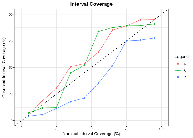
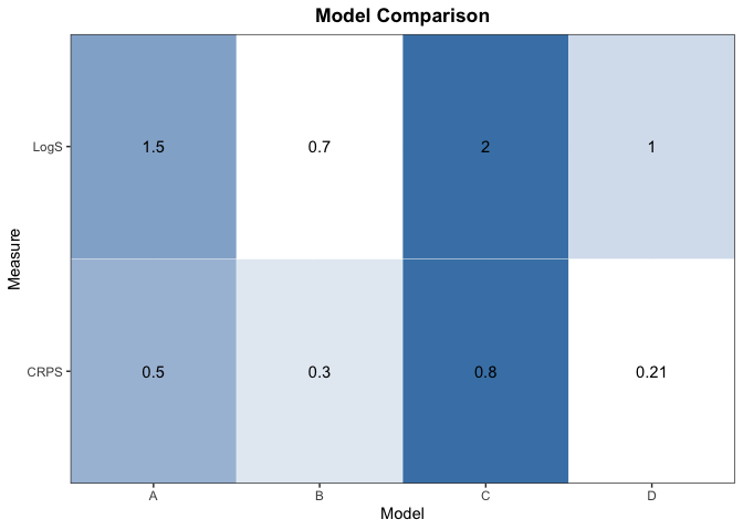
dm.test: This function performs a Diebold-Mariano-Test for two forecasts.bh.test: This function performs a Benjamini-Hochberg-Correction for different p-values.ss: This function calculates the skill score.cpi.plot: This function plots the central prediction intervals for a certain interval range.cov.plot: This function plots the central prediction interval coverage for certain interval ranges of different models.score.plot: This function plots scores of different models rated by selected measures as heatmap.
# load R package
library(eppverification)

# set.seed for reproducibility
set.seed(2023)# simulated data
n <- 30
m <- 50
y <- rnorm(n)
x <- matrix(rnorm(n*m), ncol = m)
# Verification Rank Histogram
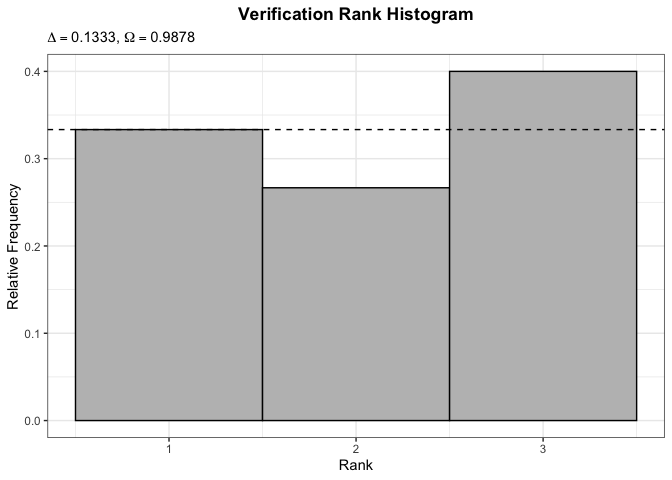
vr.hist(y = y, x = x, bins = 3, reliability = TRUE, entropy = TRUE)# simulated data
n <- 10000
u <- runif(n)
# PIT Histogram
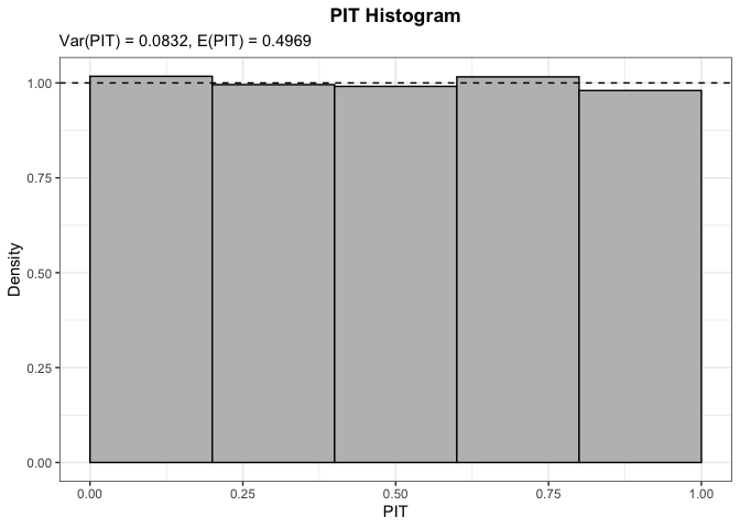
pit.hist(u = u, bins = 5, dispersion = TRUE, bias = TRUE)# Root Mean Variance
rmv(x = x)
#> [1] 1.000718# simulated data
n <- 30
m <- 50
y <- rnorm(n)
x <- matrix(rnorm(n*m), ncol = m)
# Continuous Ranked Probability Score
crps(y = y, x = x, method = "ens", aggregate = mean)
#> [1] 0.5128893# simulated data
n <- 30
y <- rnorm(n, mean = 1:n)
nominal.coverage <- 90
alpha <- (100-nominal.coverage)/100
lower <- qnorm(alpha/2, rnorm(n, mean = 1:n))
upper <- qnorm((1-alpha/2), rnorm(n, mean = 1:n))
# Central Prediction Interval Values
cpi(y = y, lower = lower, upper = upper, nominal.coverage = nominal.coverage,
separate = c("is", "overprediction", "underprediction", "width", "coverage"), aggregate = mean)
#> $is
#> [1] 7.615486
#>
#> $overprediction
#> [1] 1.813372
#>
#> $underprediction
#> [1] 2.248097
#>
#> $width
#> [1] 3.554018
#>
#> $coverage
#> [1] 0.7666667# simulated data
n <- 30
m <- 50
y <- cbind(rnorm(n), rgamma(n, shape = 1))
x <- array(NA, dim = c(m, 2, n))
x[, 1, ] <- rnorm(n*m)
x[, 2, ] <- rgamma(n*m, shape = 1)
# Multivariate Verification Rank Histogram
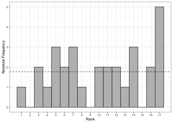
mvr.hist(y = y, x = x, method = "mv", type = "absolute", bins = 17)# simulated data
n <- 30
m <- 50
x <- array(NA, dim = c(2, 2, n))
for (i in 1:n) {
x[, , i] <- cov(cbind(rnorm(m), rgamma(m, shape = 1)))
}
#Determinant Sharpness
ds(x = x, covmat = TRUE, aggregate = mean)
#> [1] 0.9970074# simulated data
n <- 30
m <- 50
y <- cbind(rnorm(n), rgamma(n, shape = 1))
x <- array(NA, dim = c(m, 2, n))
x[, 1, ] <- rnorm(n*m)
x[, 2, ] <- rgamma(n*m, shape = 1)
# Energy Score
es(y = y, x = x, method = "ens", aggregate = mean)
#> [1] 0.6946325
# Euclidean Error
ee(y = y, x = x, method = "median", aggregate = mean)
#> [1] 0.9880346# simulated data
n <- 365
s1 <- arima.sim(list(ar = 0.7), sd = 0.5, 100)
s2 <- arima.sim(list(ar = 0.7), sd = 0.5, 100) - 0.2
p <- runif(100, min = 0, max = 0.05)
# Diebold-Mariano-Test
dm.test(s1, s2, alternative = "two.sided", h = 1)
#>
#> Diebold-Mariano Test
#>
#> data: structure(c(0.238720526066842, -0.527731263294478, 0.311552661923538, structure(c(-1.49070630436772, -0.470353701613745, -0.260411676944677, 0.236827548944262, 0.0857392854365571, -0.151746773147548, 0.3211711439308, -0.250677968228971, -0.550828354657908, -0.0243846724857634, 0.578647655516504, 0.915498650915109, 0.878214074203563, 0.782945904920966, -0.679460005400524, -0.639466429573929, -0.886710774234045, -0.844631725008147, 0.355672164990754, 0.248764487478872, 0.19276150492605, -0.887603739675973, -0.89572956260365, -0.420039243234284, -0.448139126388044, 0.223373919032025, -0.959368452736523, -0.965827971634405, -0.715084974663628, -0.765492022877302, 0.290090047902623, -0.190643969904708, 0.0927932799963356, -0.253956765739785, -0.786653123719523, -1.0643575389332, -0.859129420461269, 0.147016067759562, -0.875473920889236, -0.723519893485028, -1.85011875511786, -1.42757321627682, 0.591712226844409, 1.38529782490813, 1.50768374890694, 1.70536760672312, -0.752472561151255, 0.71524294869209, 0.204427788057569, 0.0486886569929789, 1.30844661115758, 0.866720778145616, 1.04606621853937, 0.471187225896344, -0.034950687117501, 0.0361193966601754, 0.0613577397987986, 0.0577593105559278, 0.460826075184299, -0.463840530429393, 0.0905109451028114, 0.523580359536329, 0.0166040959303252, 0.228957811267457, 0.0371157653754927, 0.273246214303869, 1.29250669508678, 0.91799192851402, 0.46013187475581, 0.50809666155914, 0.00327177466431558, 0.0930170758912109, -0.729345866722121, 0.0435873251694169, 0.163987942873975, -0.385880513240643, 0.433841888622072, -0.628638560363066, 0.0198554276187063, -1.03896262329088, -1.37823750811594, 0.400041755866377, 0.557267334237013, 0.260244578797202, -0.142888252192723, -2.04661543997303, -1.26358801824628, -0.722194283127594, 0.539418916186468, 0.0376458013486344, -0.0666367311277612, -0.607937745232438, 0.104122688367564, 1.07008213421922, -0.0520742385014142, -0.384898930980601, -0.475742444606428, -0.296598415455014, -0.120696628666513, -0.164331193002039, -0.879493672430848, -1.09696703423004, -0.852620583035503, -0.53376983451821, -0.271614232599621, -0.527404564926944, -0.451509694482224, -0.3051251351083, -1.01386196516451, -0.425201968238743, 0.0856001189929098, 0.102355572020975, -0.579815471402505, -0.463970166149353, -1.31278499319737, -0.573466108858527, -0.0608194536647661, 0.617509824372005, 0.548583091418607, 0.534804529954491, -0.866119570965604, -0.948031199948479, -1.28321667477519, -1.02355251051274, 1.26007118596867, 0.811702233037451, 0.563206731453456, 0.290718106644499, -0.483526154294208, -0.457240488223711, 0.496702512218391, 0.80793753719876, 0.15587100656237, -0.232761599140489, -0.673453914318467, -0.651448901019745, 0.693771933262046, 0.257364705306704, -0.27207965707141, 0.153465233424303, -0.392951412147586, -0.637245150589652, -0.496622963442796, -0.722011950019451, 0.351605745705148, 0.306368695124342, 0.389678976144498, 0.209344276430475, -1.26026704741524, -0.629868121494733, -0.989053267515073, -0.446763031725633, -0.427561937080649, 0.16032909520674, -0.285677038421974, -1.01903393031835, -0.464854912482491, -0.330717432789186, 0.928952685560274, 0.805647019017016, -0.366558495300433, 0.707467311984842, 0.907509267347139, 0.668129826095563, 0.973023286621081, 1.83416975602533, 0.989947815528484, 0.722767402917373, 0.307640999616576, -0.549413457422668, -1.02721107666597, -0.382173760704628, 0.931875374570217, 0.14974631793673, 0.241121068157678, 0.0143858743788231, 0.409488701203636, -0.667870538511744, -0.769790304737059, -0.517839123234736, -0.285182686245866, -0.947961861244806, -1.43749993478763, -0.662670344526401, -1.07869433307153, -1.63976688831352, -0.480737245736788, -0.58824759530726, -0.428041838775768, -1.61117402497825, -1.73157944258176, -1.3213869359581, -0.754352488020815, -0.922002572144512), tsp = c(1, 100, 1), class = "ts") -0.367306288312317, -0.0923894434372354, -0.333204000312379), tsp = c(1, structure(c(0.238720526066842, -0.527731263294478, 0.311552661923538, 100, 1), class = "ts")
#> DM = 2.3809, Forecast Horizon = 1, p-value = 0.01727
#> alternative hypothesis: two.sided
# Benjamini-Hochberg-Procedure
bh.test(p, alpha = 0.05)
#> [1] TRUE TRUE TRUE TRUE TRUE TRUE TRUE TRUE TRUE TRUE TRUE TRUE TRUE TRUE TRUE
#> [16] TRUE TRUE TRUE TRUE TRUE TRUE TRUE TRUE TRUE TRUE TRUE TRUE TRUE TRUE TRUE
#> [31] TRUE TRUE TRUE TRUE TRUE TRUE TRUE TRUE TRUE TRUE TRUE TRUE TRUE TRUE TRUE
#> [46] TRUE TRUE TRUE TRUE TRUE TRUE TRUE TRUE TRUE TRUE TRUE TRUE TRUE TRUE TRUE
#> [61] TRUE TRUE TRUE TRUE TRUE TRUE TRUE TRUE TRUE TRUE TRUE TRUE TRUE TRUE TRUE
#> [76] TRUE TRUE TRUE TRUE TRUE TRUE TRUE TRUE TRUE TRUE TRUE TRUE TRUE TRUE TRUE
#> [91] TRUE TRUE TRUE TRUE TRUE TRUE TRUE TRUE TRUE TRUE# simulated data
n <- 30
x <- seq(Sys.Date(), by = "day", length.out = n)
y <- rnorm(n, mean = 1:n)
nominal.coverage <- 90
alpha <- (100-nominal.coverage)/100
lower <- qnorm(alpha/2, rnorm(n, mean = 1:n))
upper <- qnorm((1-alpha/2), rnorm(n, mean = 1:n))
# Central Prediction Intervals Plot
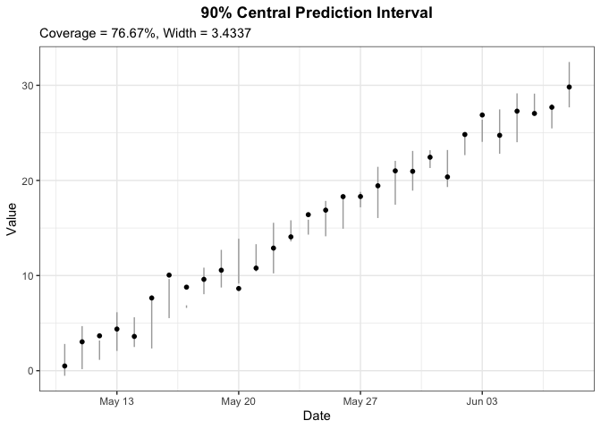
cpi.plot(x = x, y = y, lower = lower, upper = upper, nominal.coverage = nominal.coverage, x.lab = "Date", y.lab = "Value", info = TRUE)# simulated data
n <- 30
x <- matrix(runif(n)*100, ncol = 3)
x <- apply(x, 2, sort)
nominal.coverage <- seq(5, 95, length.out = 10)
models <- c("A", "B", "C")
# Central Prediction Interval Coverage Model Comparison
cov.plot(x = x, models = models, nominal.coverage = nominal.coverage)# simulated data
x <- matrix(c(0.5, 0.3, 0.8, 0.21, 1.5, 0.7, 2, 1), byrow = TRUE, ncol = 4)
models <- c("A", "B", "C", "D")
measures <- c("CRPS", "LogS")
# Score Plot
score.plot(x = x, models = models, measures = measures)Feel free to contact jobstd@uni-hildesheim.de if you have any questions or suggestions.
Gneiting, T. and Raftery, A. (2007). Strictly Proper Scoring Rules, Prediction, and Estimation. Journal of the American Statistical Association. 102(477). 359-378.


