jmineroff/Domino-Launchpad-Quickstart

Domino Tutorial: Predicting Wine Quality

In this project you will work through an end-to-end workflow broken into various labs to:

Read in data from a live source
Prepare your data in an IDE of your choice, with an option to leverage distributed computing clusters
Train several models in various frameworks
Compare model performance across different frameworks and select best performing model
Deploy model to a containerized endpoint and web-app frontend for consumption
Leverage collaboration and documentation capabilities throughout to make all work reproducible and sharable!

Section 1 - Project Set Up

Lab 1.1 - Forking Existing Projects

Guide your mouse to the sidebar and click the Search page. Afterwards, type the word Training in the cell provided and hit Enter to discover any projects tagged with Training. (The blue sidebar shrinks to show only the icon of the pages; unshrink it by guiding your mouse over the icon pages.)

Select the project called WineQuality.

Look at the readme to learn more about the project.

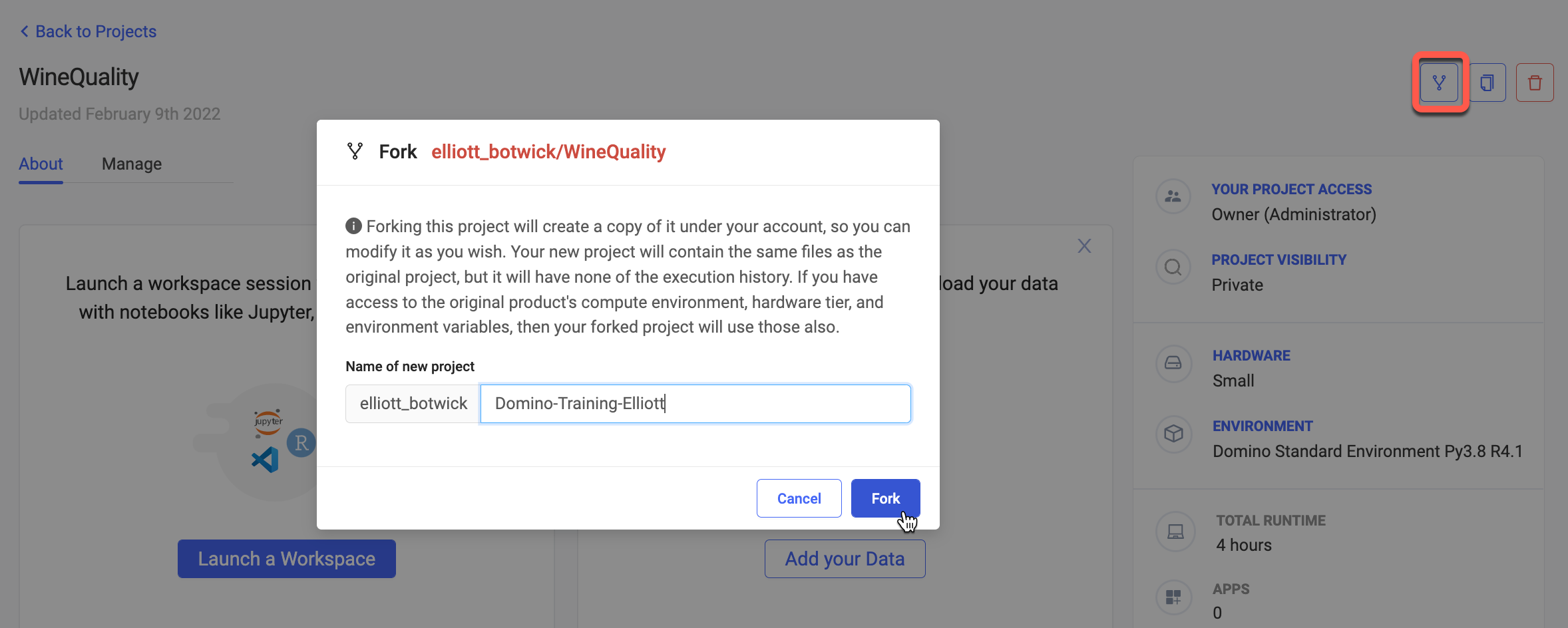
In the top right corner, choose the icon to Fork the project. Name the project WineQuality.

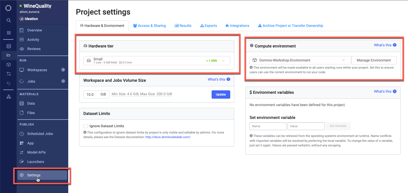
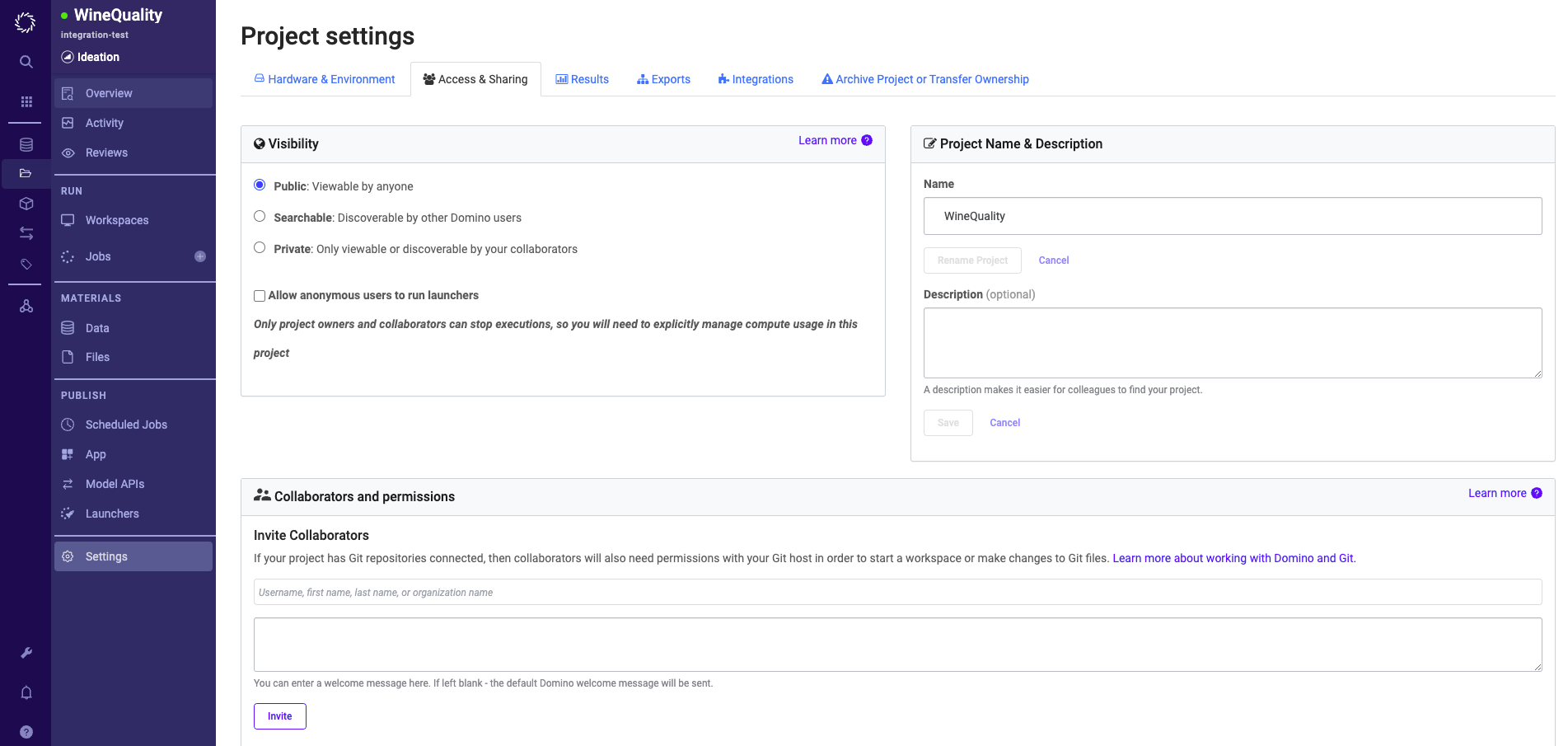
In your new project - go into the Settings tab to view the default Hardware Tier and Compute Environment - ensure they are set to Small and WineQuality respectively:

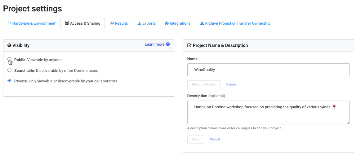
Go to the Access and Sharing tab and change your project visibility to Public. This allows anyone with access to your Domino URL to see the files and executions in your project. Note: on LaunchPad, they must first have logged in with the NVIDIA-provided credentials.

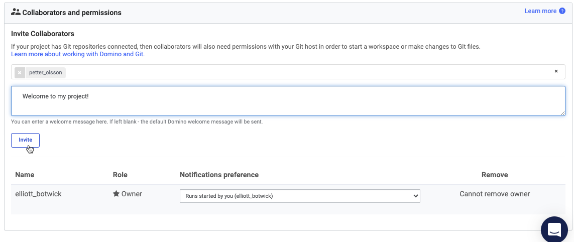
[optional] - If a colleague of yours has an account in this Domino, you can add them as a collaborator in your project.

Change their permissions to Results Consumer. This permission level does not allow them to start executions or change files in your project, but will allow them to see files and published artifacts.

Lab 1.2 - Defining Project Goals

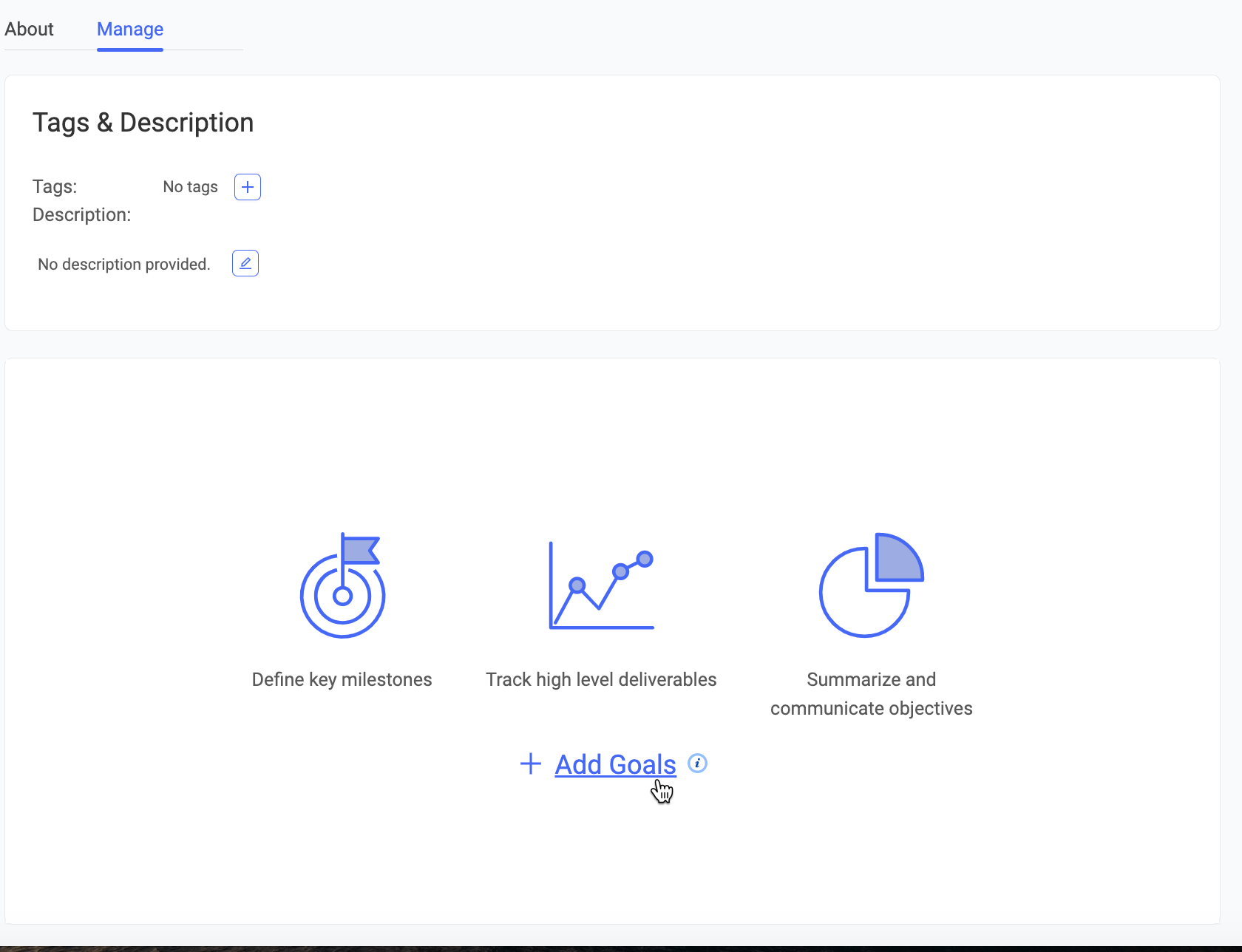
Click back into the Overview area of your project. Then navigate to the Manage tab.

Click on Add Goals.

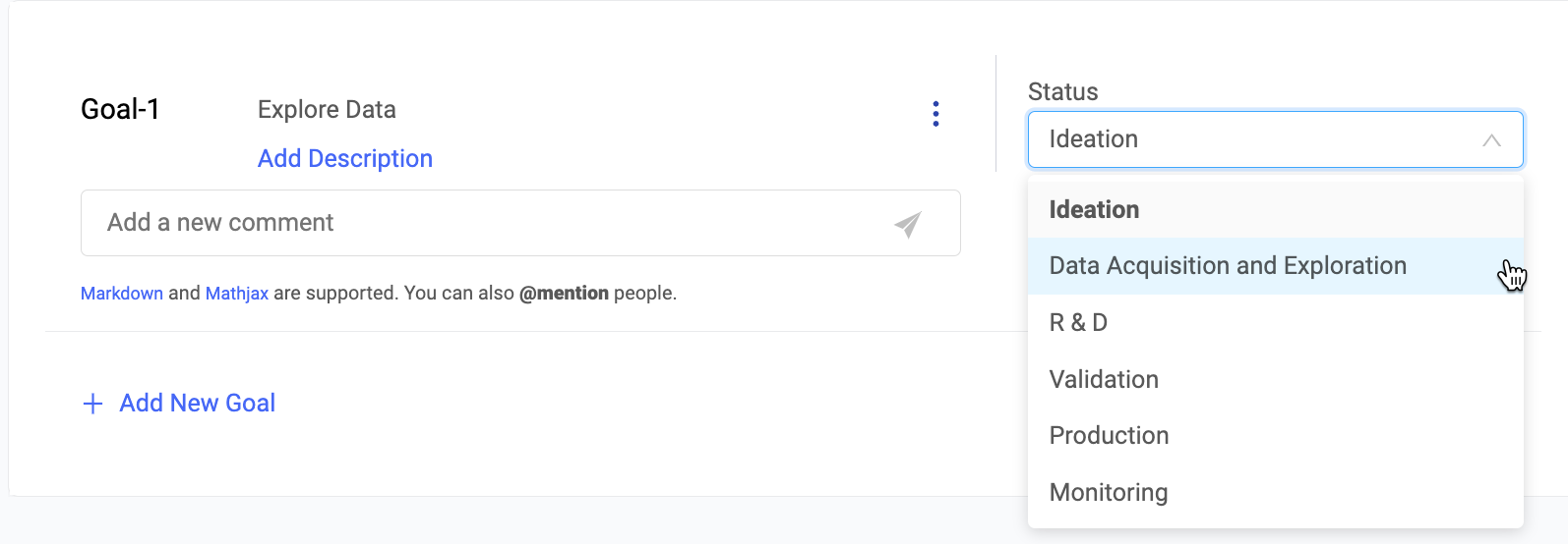
For the goal title type in Explore Data and click Save. Once the goal is saved click the drop down on the right to mark the goal status as Data Acquisition and Exploration.

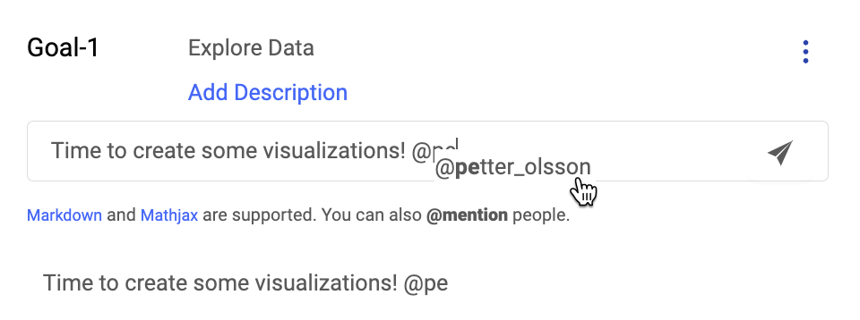
[optional] - If you've already added a collaborator to Domino, add a comment to the goal and tag them by typing '@' followed by their username. Click on the paper airplane to submit the comment.

Lab 1.3 - Add Data Source

We will now add a data connection to the project so we can query data. As a code-first platform, Domino allows you to connect to data with any Python/CLI/etc. tools you already use, but there are also UI methods that make it easier to share and manage your data sources.

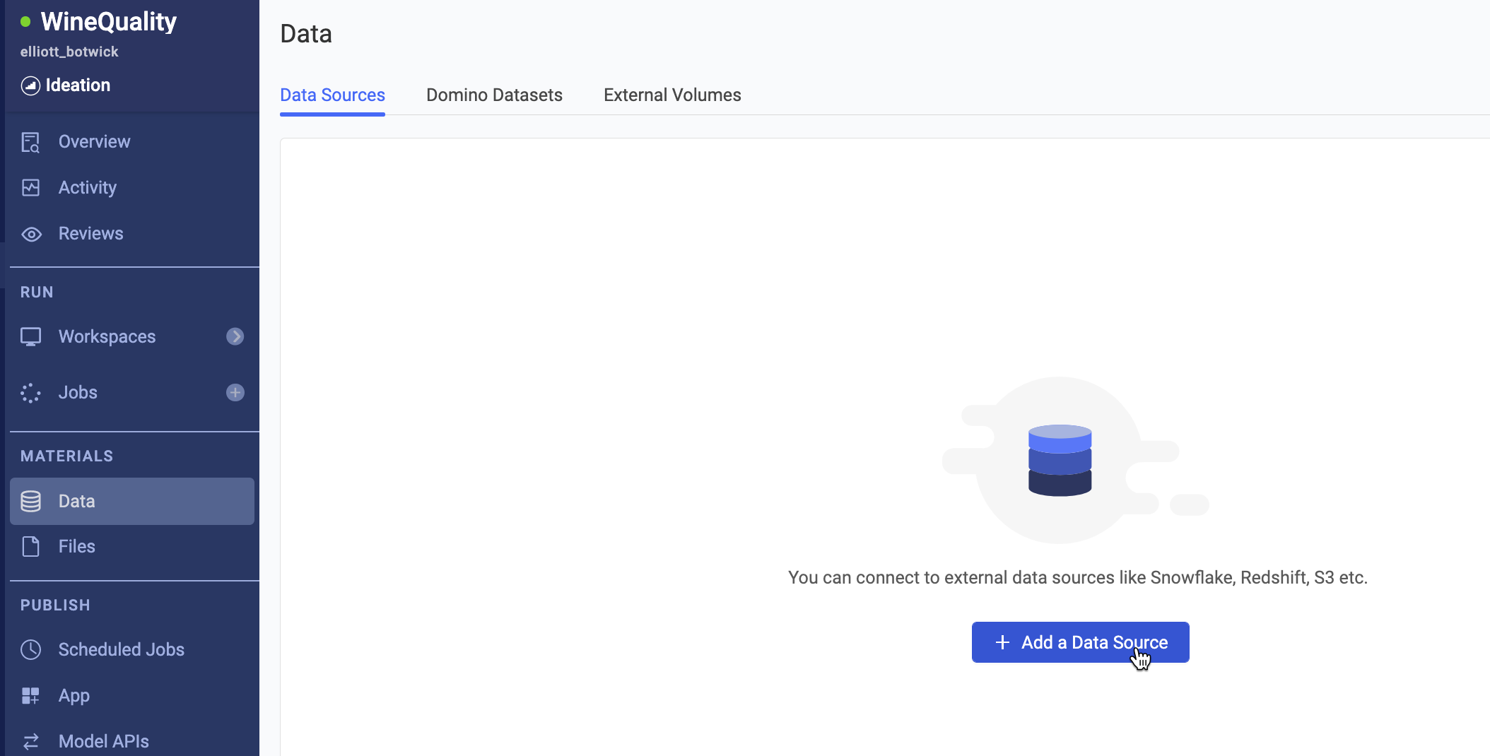
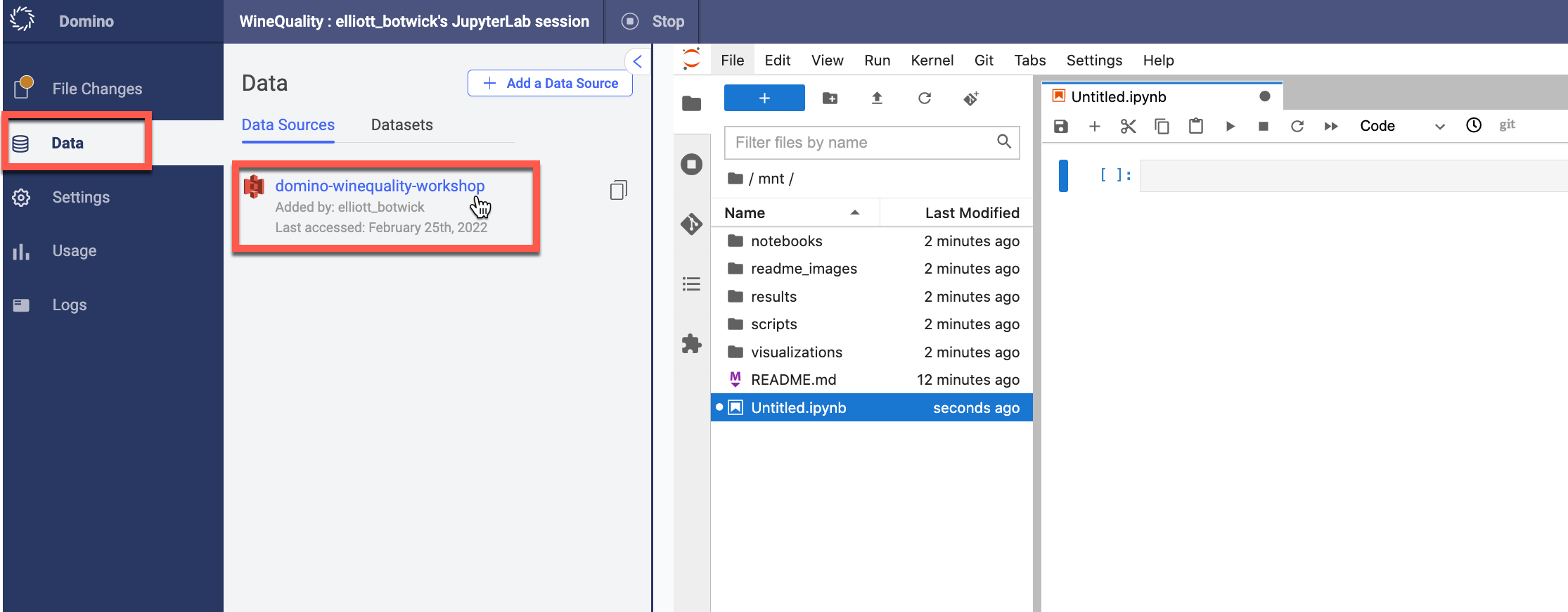
To use one of these, navigate to Data in the sidebar of your project and click on Add a Data Source (you may need to click on the Data Sources tab first).

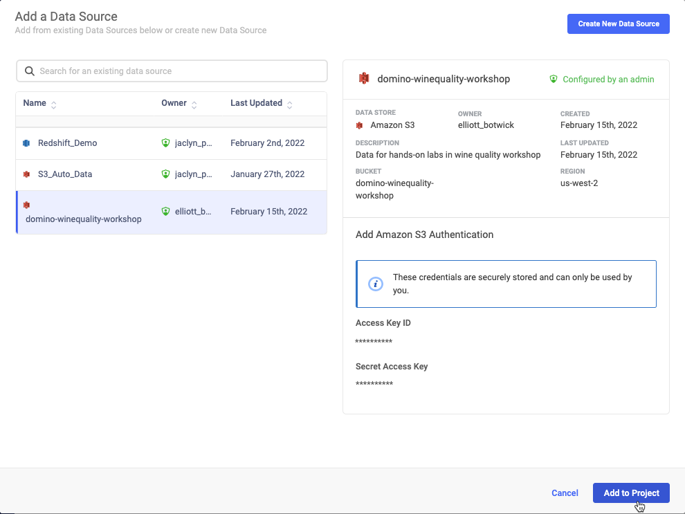
Select the WineQuality S3 bucket connection and click Add to project. This example connection was predefined by an admin, but it is possible for all users to create these.

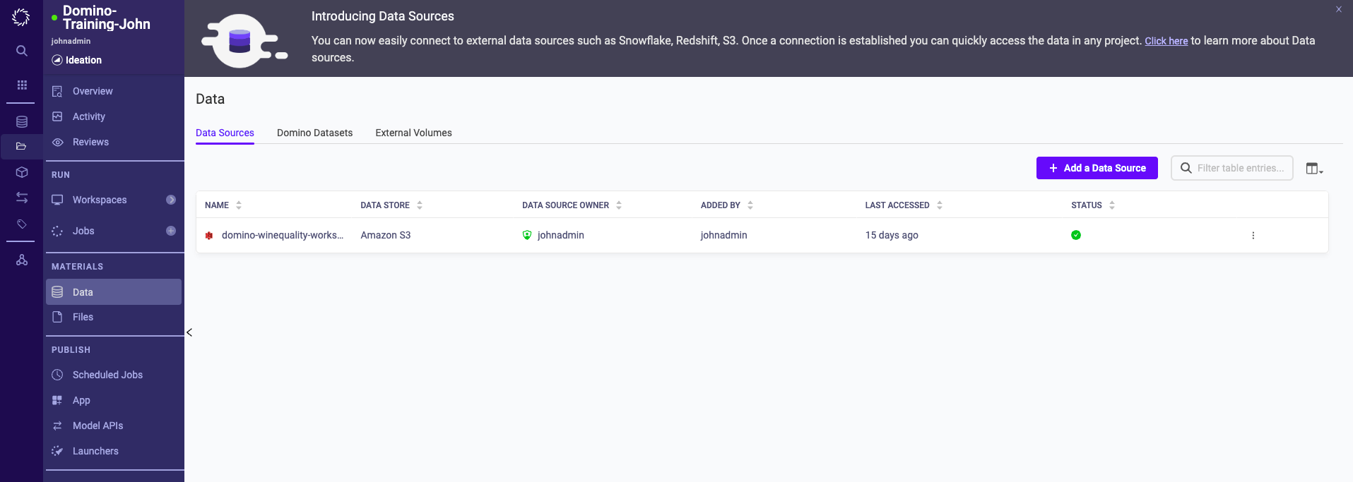
The Data Source should look like the image below.

This concludes all labs in Section 1 - Prepare Project and Data!

Section 2 - Develop Model

Now that we have our data in place, let's set up everything we need to run executions and train a model.

Lab 2.1 - Inspect Compute Environment

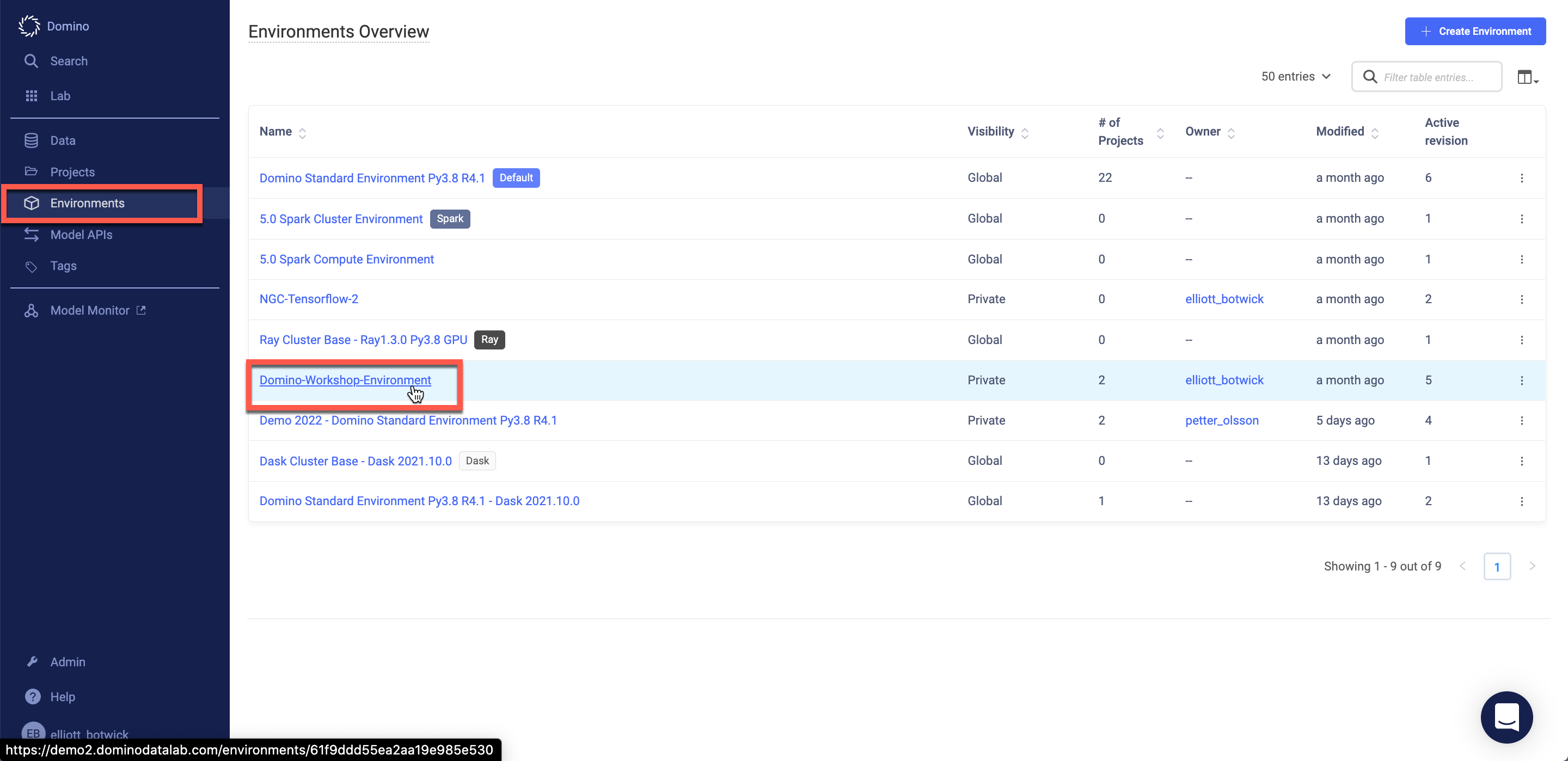
From the left blue menu click on the cube icon labelled Environments. Compute Environments are a Domino abstraction based on Docker images -- effectively a snapshot of a machine at a given point of time -- which allow you to:

Rerun code from months or years ago and know that the underlying packages/dependencies are unchanged.
Collaborate while being sure that you and your teammates are using the exact same software environment.
Cache a large number of packages so you don't have to wait for them to install the first time you (or a coworker) runs your code.

Select the WineQuality Environment.

Inspect the Dockerfile to understand the packages installed, configurations specified, and kernels installed etc.

Scroll down to Pluggable Workspaces Tools. This is the area in the Compute Environment where IDEs are made available for end users.

Scroll down to the Run Setup Scripts section. Here we have a script that executes upon startup of workspace sessions or job (pre-run script) and a script that executes upon termination of a workspace session or job (post-run script).

Finally navigate to the Projects tab - you should see all projects that are leveraging this compute environment. Click on your project to navigate back to it.

Click into the Workspaces tab to prepare for the next lab.

Lab 2.2 - Exploring Workspaces

Workspaces are interactive sessions in Domino where you can use any of the IDEs you have configured in your Compute Environment or the terminal.

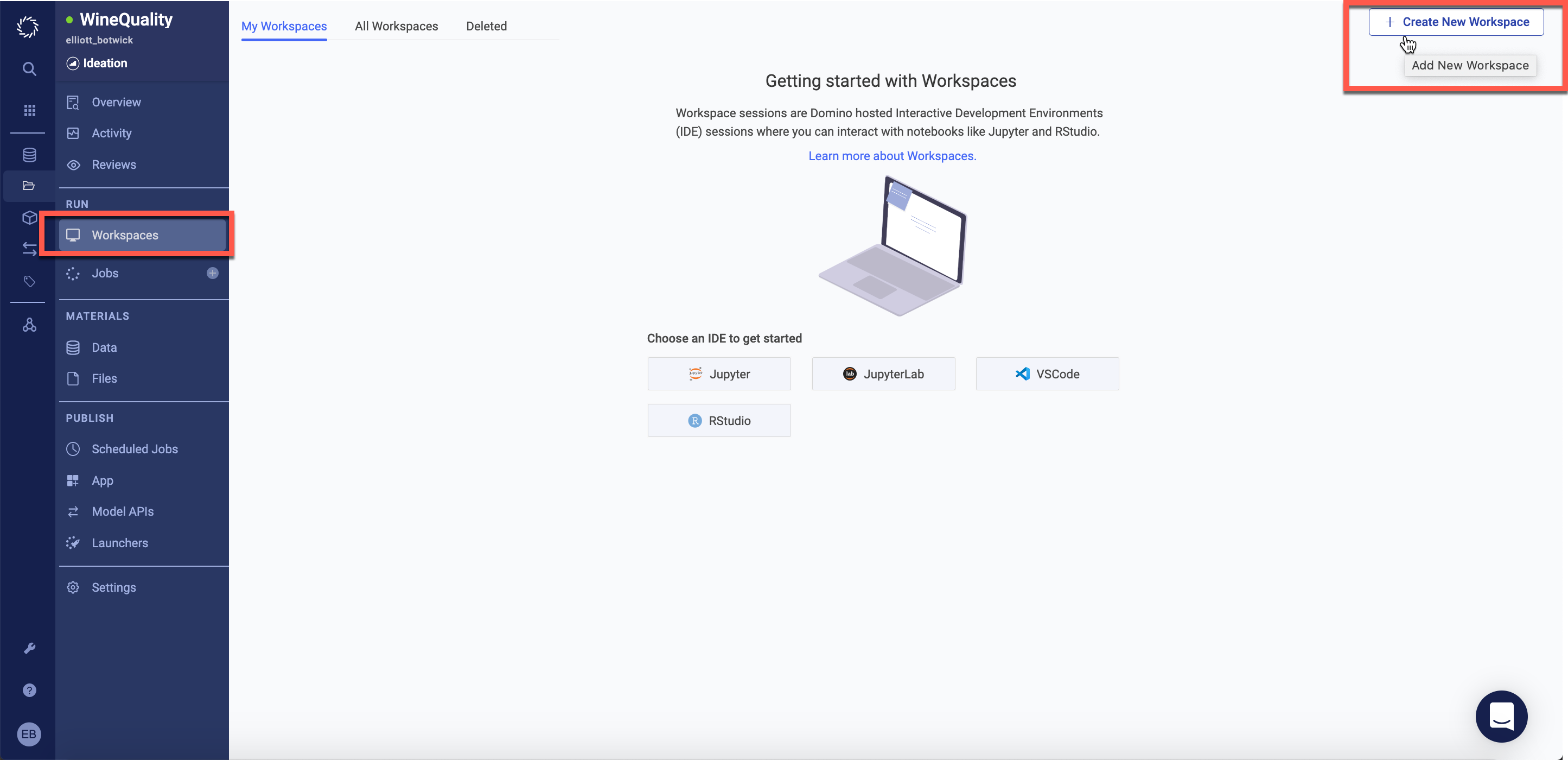
In the top right corner click Create New Workspace.

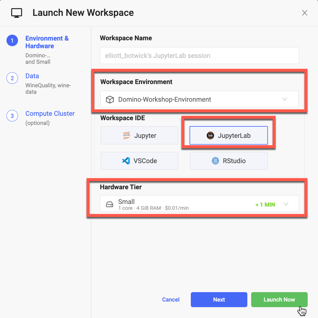
Type a name for the Workspace in the Workspace Name cell. Next, click through the available Compute Environments in the Workspace Environment dropdown and ensure that WineQuality is selected.

Select JupyterLab as the Workspace IDE.

Click the Hardware Tier dropdown to browse all available hardware configurations - ensure that Small is selected.

Click Launch now.

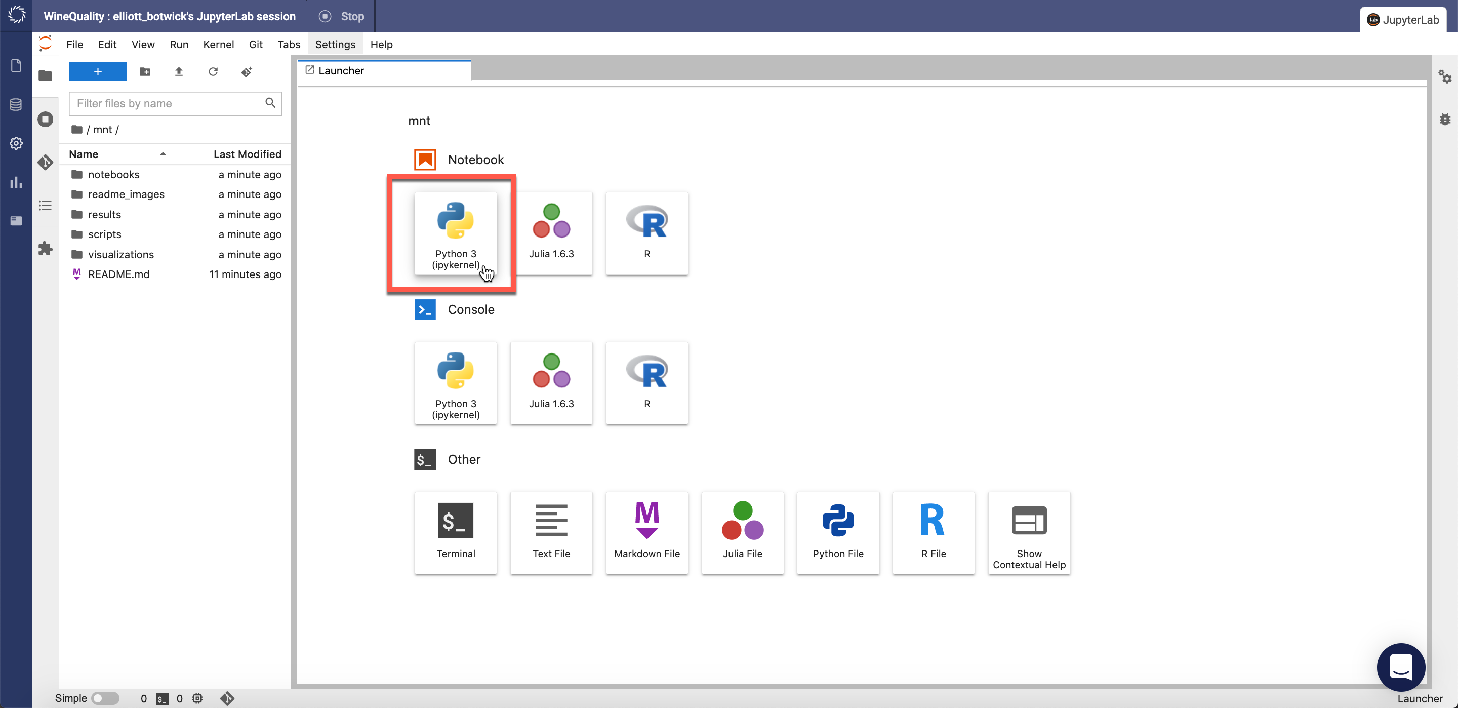
Once the workspace is launched, create a new python notebook by clicking here:

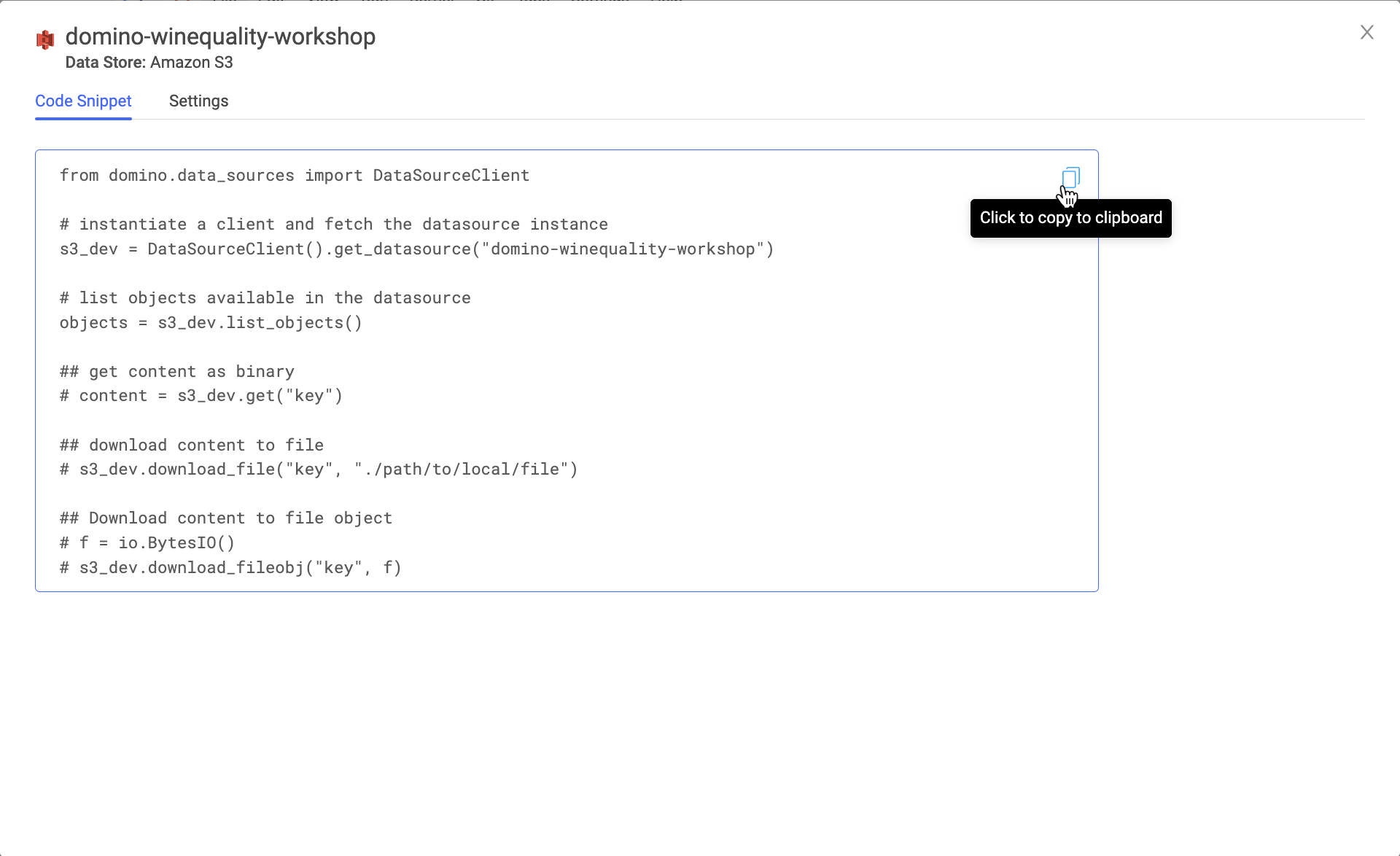
Once your notebook is loaded, click on the left blue menu and click on the Data page, followed by the Data Dource we added in Lab 1 as displayed below.

Copy the provided code snippet into your notebook and run the cell.

After running the code snippet. Copy the code below into the following cell.

from io import StringIO
import pandas as pd

s=str(object_store.get("WineQualityData.csv"),'utf-8')
data = StringIO(s) 

df=pd.read_csv(data)
df.head()

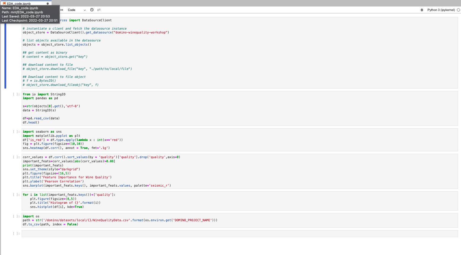
Now, copy the code snippets below cell-by-cell and run the cells to visualize and prepare the data! (You can click on the + icon to add a blank cell after the current cell).

import seaborn as sns
import matplotlib.pyplot as plt
df['is_red'] = df.type.apply(lambda x : int(x=='red'))
fig = plt.figure(figsize=(10,10))
sns.heatmap(df.corr(), annot = True, fmt='.1g')

corr_values = df.corr().sort_values(by = 'quality')['quality'].drop('quality',axis=0)
important_feats=corr_values[abs(corr_values)>0.08]
print(important_feats)
sns.set_theme(style="darkgrid")
plt.figure(figsize=(16,5))
plt.title('Feature Importance for Wine Quality')
plt.ylabel('Pearson Correlation')
sns.barplot(important_feats.keys(), important_feats.values, palette='seismic_r')

for i in list(important_feats.keys())+['quality']:
    plt.figure(figsize=(8,5))
    plt.title('Histogram of {}'.format(i))
    sns.histplot(df[i], kde=True)

Finally write your data to a Domino Dataset by running. Domino Datasets are read-write folders that allow you to efficiently store large amounts of data and share it across projects. They support access controls and the ability to create read-only snapshots, but those features are outside the scope of this lab.

import os
path = str('/domino/datasets/local/{}/WineQualityData.csv'.format(os.environ.get('DOMINO_PROJECT_NAME')))
df.to_csv(path, index = False)

Your notebook should now be populated like the display below.

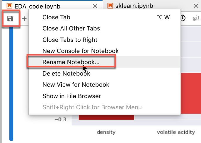
Rename your notebook EDA_code.ipynb by right clicking on the file name as shown below then click the save icon.

Lab 2.3 - Syncing Files

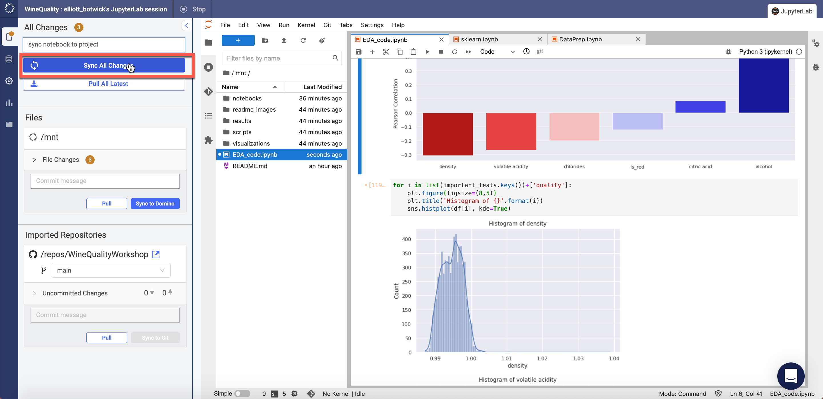
Files in a workspace are seperate from the files in your project. Now that we've finished working on our notebook, we want to sync our latest work. To do so click on the File Changes tab in the top left corner of your screen.

Enter an informative but brief commit message such as Completed EDA notebook and click Sync All Changes.

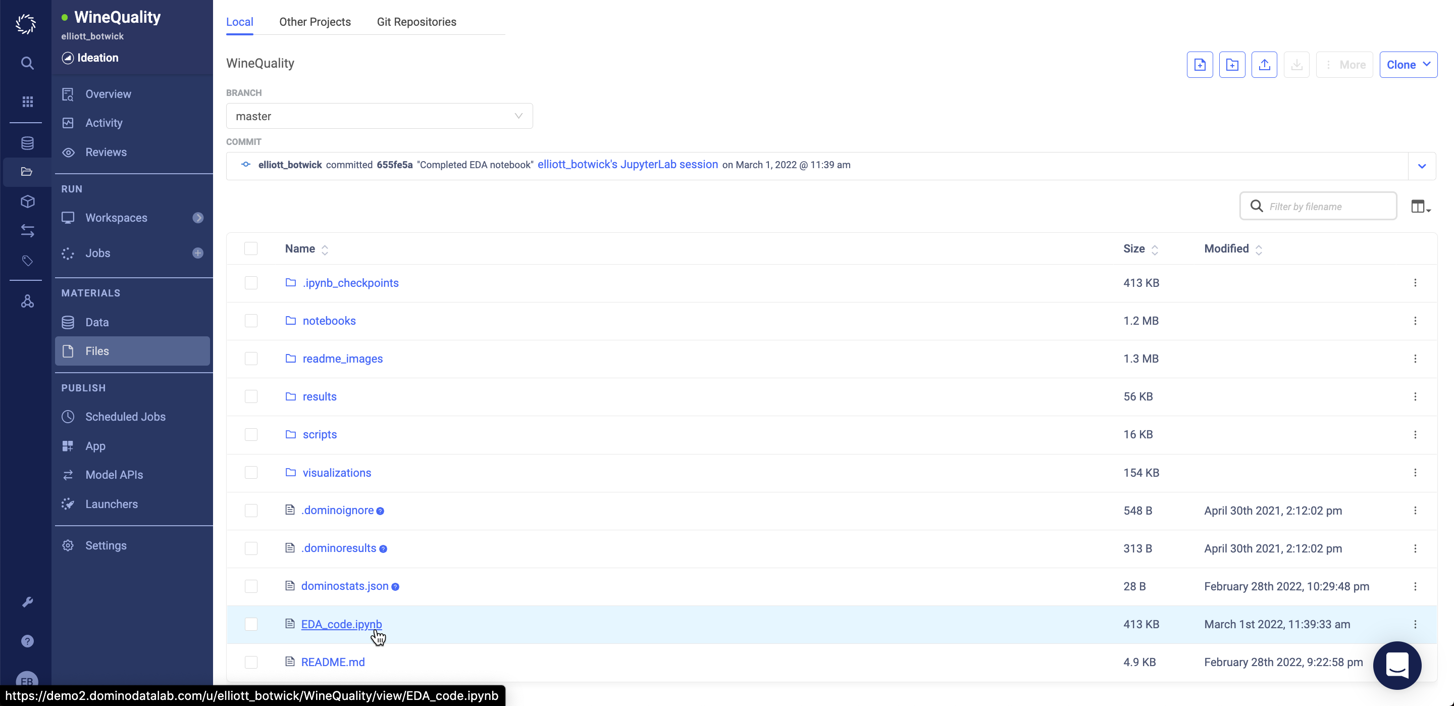
Click the Domino logo on the upper-left corner of the blue menu and select the Project page. Then select your project followed by selecting Files on the blue sidebar as shown below.

Notice that the latest commit will reflect the commit message you just logged and you can see EDA_code.ipynb in your file directory.

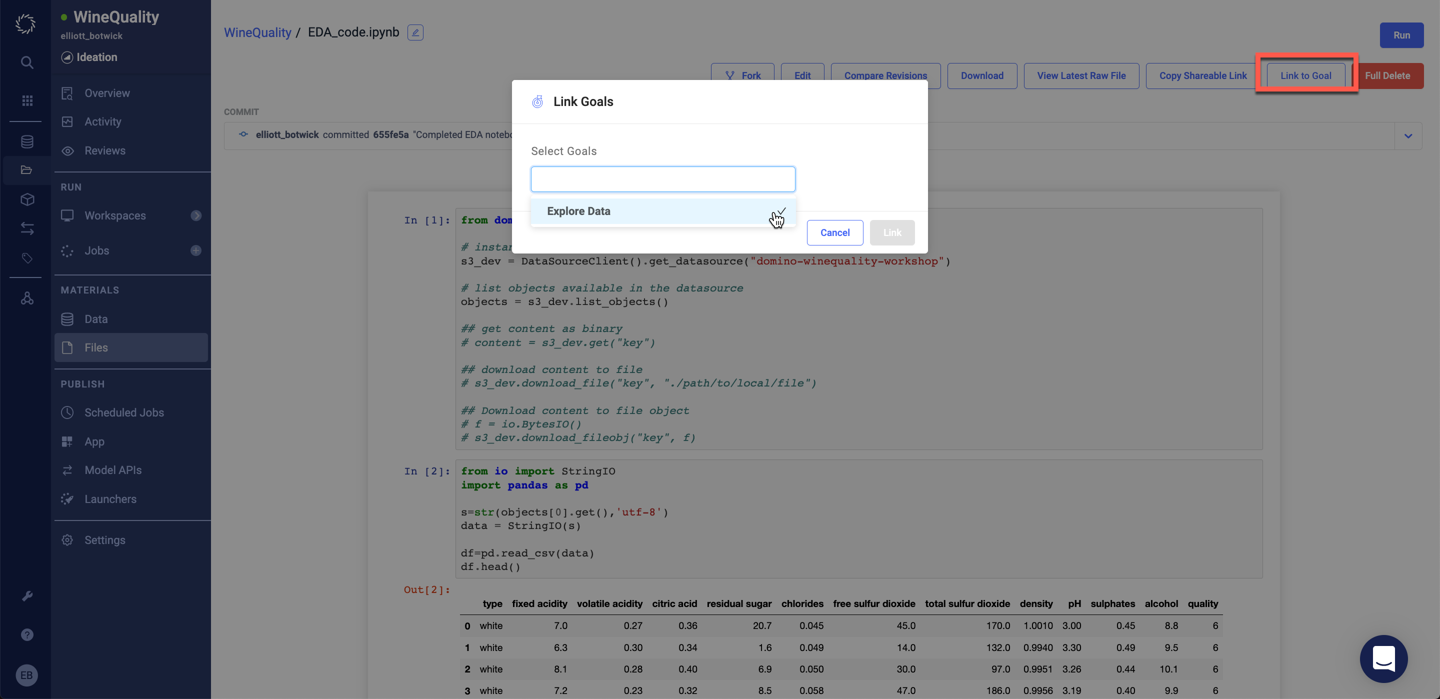
Click on your notebook to view it. On the top of your screen and click Link to Goal in the dropdown and then select the goal you created in Lab 1.2.

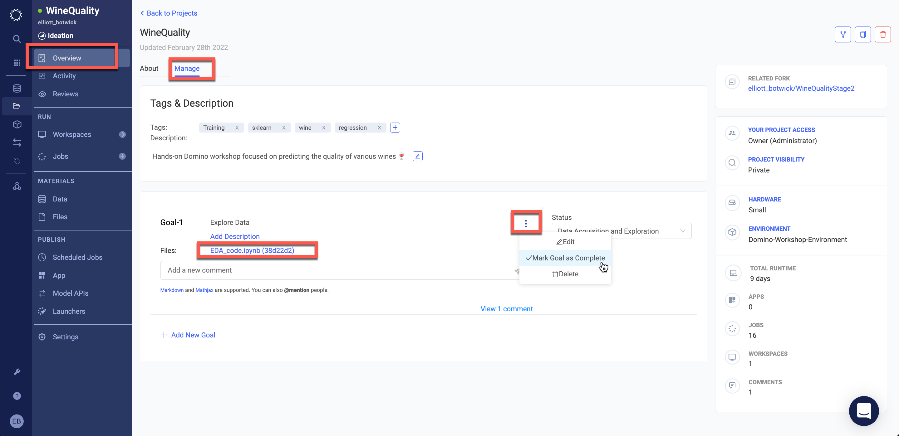
Now navigate to Overview and the Manage tab to see your linked notebook.

Click the ellipses on the goal to mark the goal as complete.

Lab 2.4 - Run and Track Experiments

Now it's time to train our models!

We are taking a three pronged approach and building a model in sklearn (python), xgboost (R), and an auto-ml ensemble model (h2o).

First, navigate back to your JupyterLab workspace tab. In your file browser go into the scripts folder and inspect multitrain.py.

Check out the code in the script and comments describing the purpose of each line of code.

You can also check out any of the training scripts that multitrain.py will call.

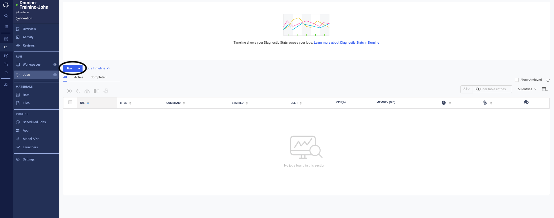
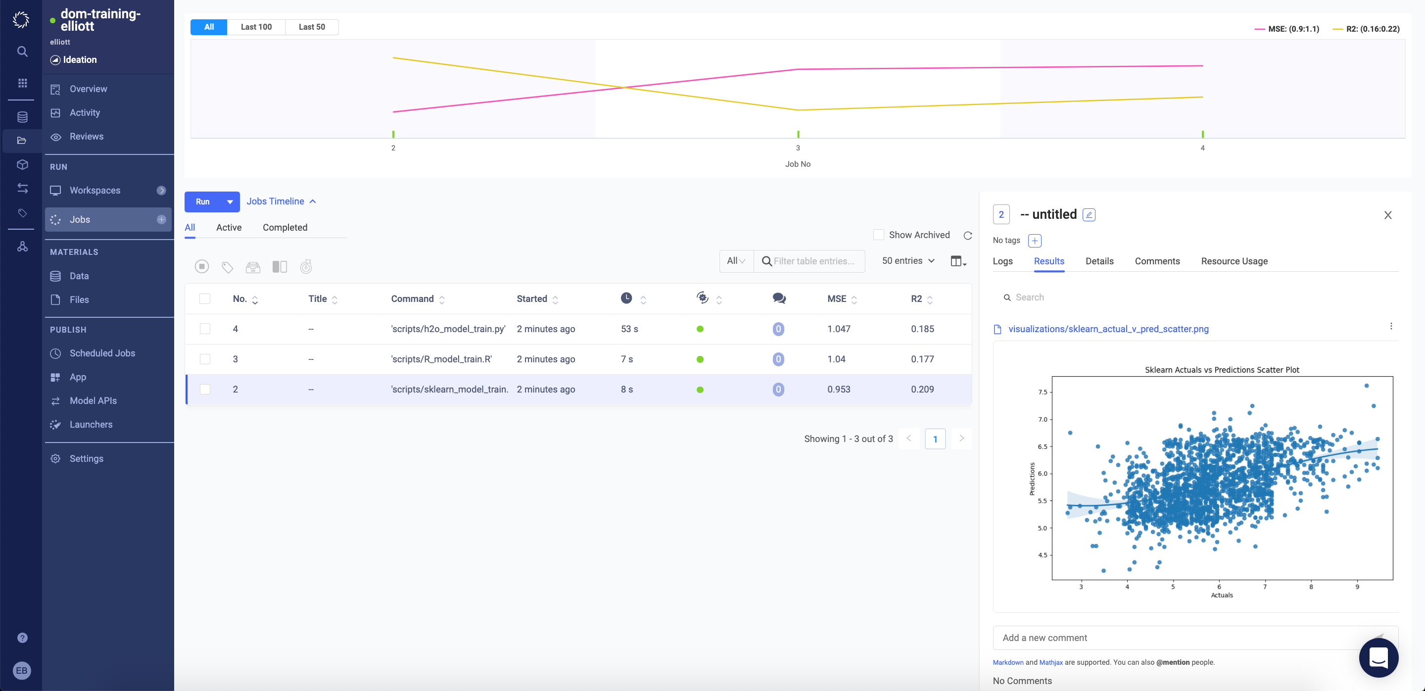
Now switch into your other browser tab to return to your Domino Project. Navigate to the Jobs page. Domino Jobs are non-interactive workloads that run a script in your project. While Workspaces stay open for an arbitrary amount of time (within admin-defined limits), Jobs will free up the underlying compute resources as soon as the script execution is finished.

Click on Run.

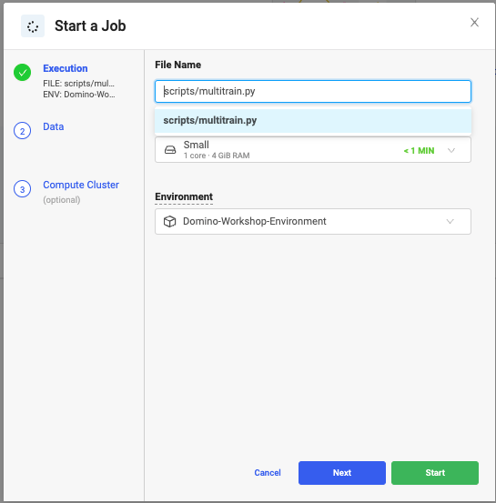
Type in the following command in the File Name section of the Start a Job pop-up window. Click on Start to run the job.

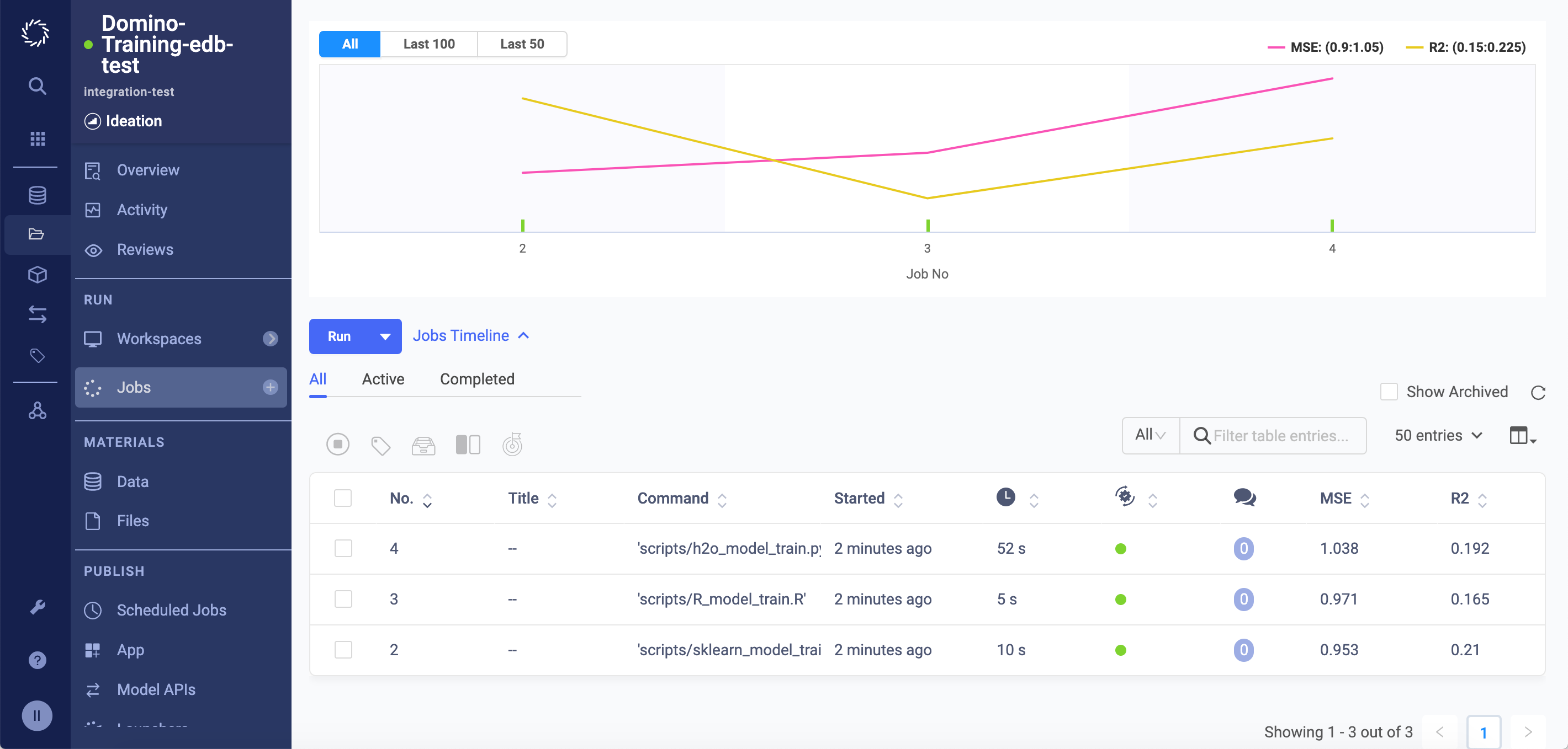
scripts/multitrain.py

Watch as three job runs have appeared, you may see them in starting, running or completed state.

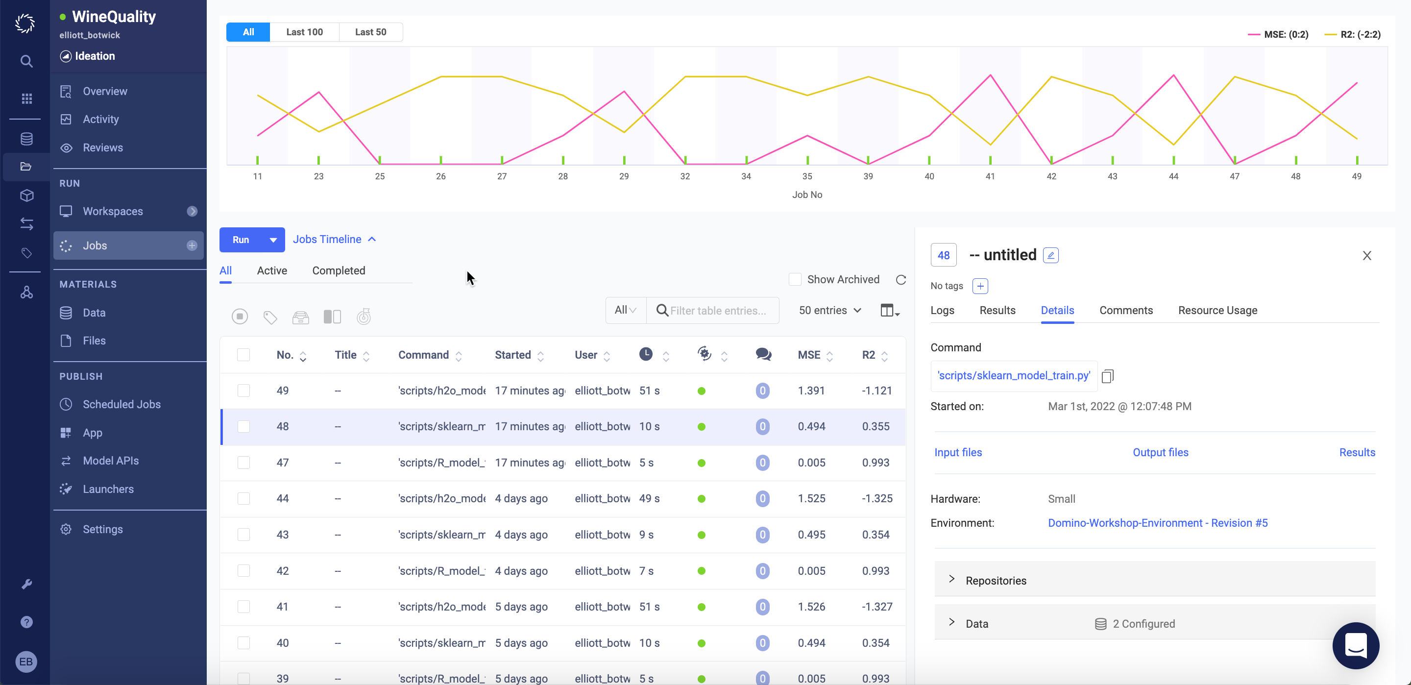
Click into the sklearn_model_train.py job run.

In the Details tab of the Job, note that the Compute Environment and Hardware Tier are tracked to document not only who ran the experiment and when, but what versions of the code, software, and hardware were executed.

Click on the Results tab of the Job. Scroll down to view the visualizations and other outputs.

We've now trained 3 models and it is time to select which model we'd like to deploy.

Refresh the page. Inspect the table and graph to understand the R^2 value and Mean Squared Error (MSE) for each model. From our results it looks like the sklearn model is the best candidate to deploy.

In the next section of labs we will deploy the model we trained here!

Section 3 - Deploy Model

Lab 3.1 Deploying Model API Endpoint

Now that you have completed model training and selection - it's time to get your model deployed.

In the last lab - we trained a sklearn model and saved it to a serialized (pickle) file. We now want to deploy the trained model using a script to load in the saved model object and pass new records for inference.

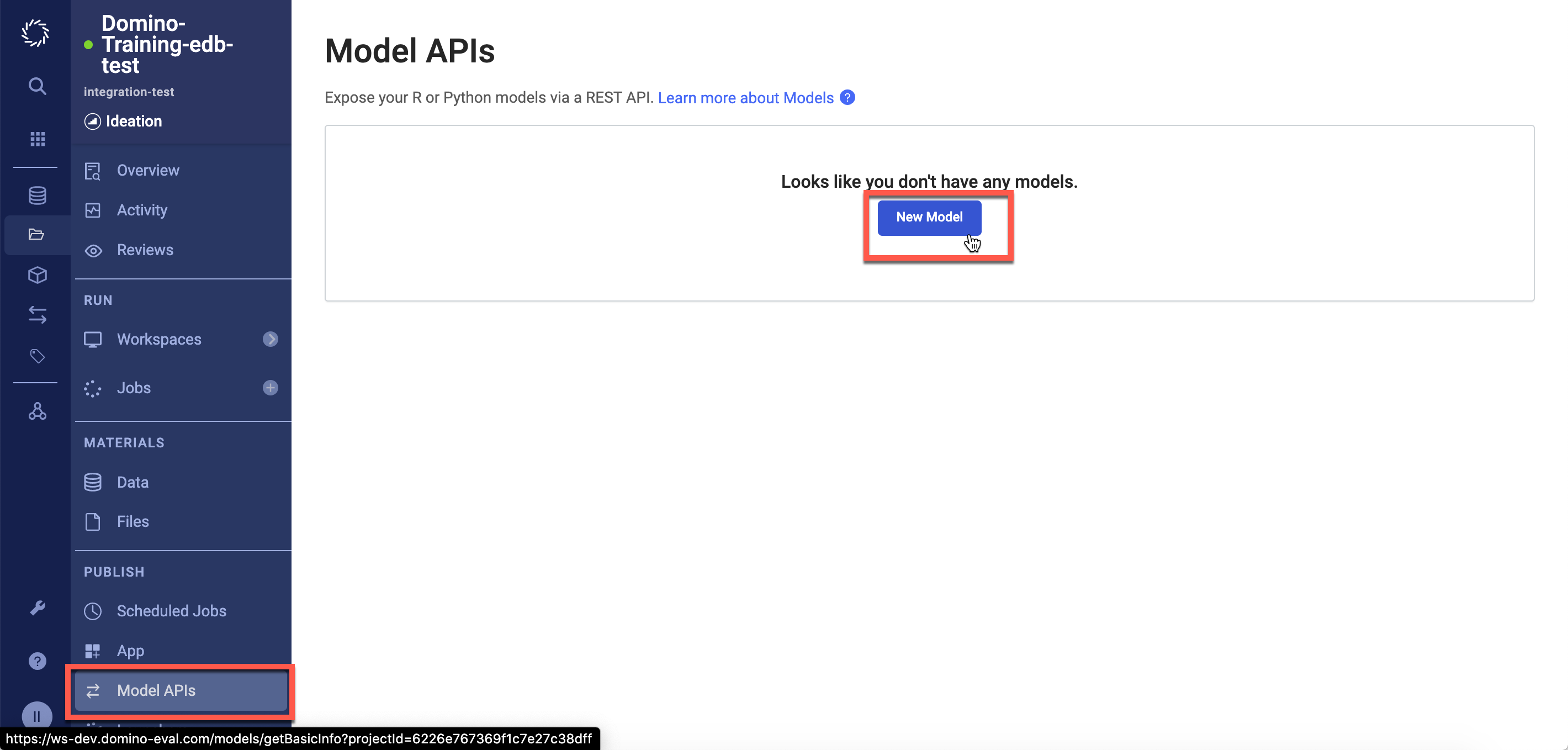
To do so - navigate to the Model APIs tab in your project. Click New Model.

Name your model wine-quality-yourname

For the description add the following:

Model Endpoint to determine the quality of wine

Sample Scoring Request: 
    
{
  "data": {
    "density":0.99,
    "volatile_acidity": 0.028,
    "chlorides": 0.05 ,
    "is_red":0,
    "alcohol": 11
  }
}

Be sure to check the box Log HTTP requests and responses to model instance logs.

Click Next. On the next page:

For Choose an Environment select WineQuality

For The file containing the code to invoke (must be a Python or R file) enter scripts/predict.py

For The function to invoke enter predict

And click Create Model.

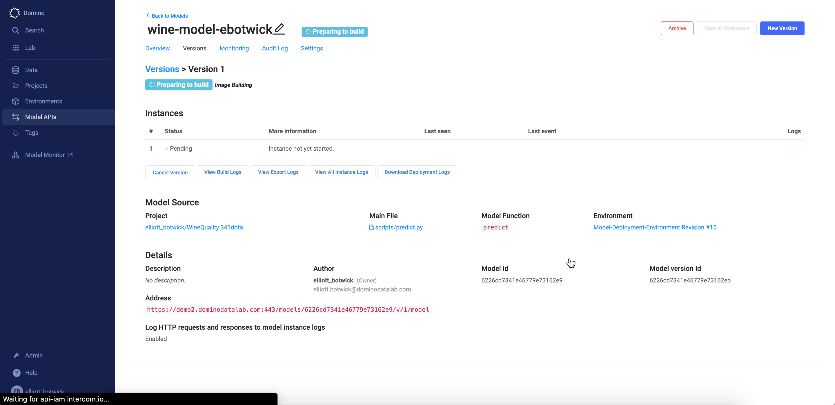
Over the next 2-5 minutes, you'll see the status of your model go from Preparing to Build -> Building -> Starting -> Running.

Domino is creating a new Docker image that includes the files in your project, your compute environment, and additional code to host your script as an API. Once your model reaches the Running state -- a pod containing your model object and code for inference is up and ready to accept REST API calls.

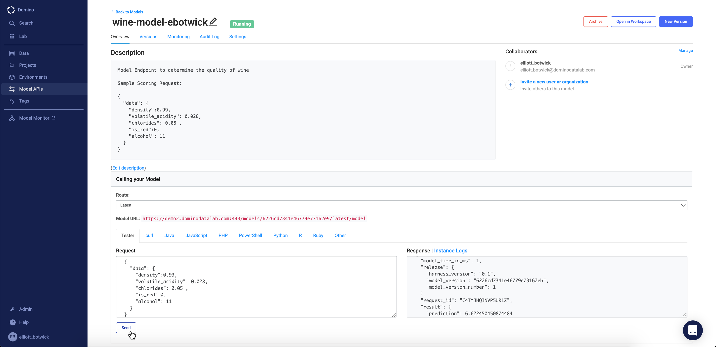
To test your model navigate to the Overview tab. In the Request field in the Tester tab enter a scoring request in JSON form. You can copy the sample request that you defined in your description field.

In the Response box you will see a prediction value representing your model's predicted quality for a bottle of wine with the attributes defined in the Request box. Try changing 'is_red' from 0 to 1 and 'alcohol' from 11 to 5 to see how the predicted quality differs. Feel free to play around with different values in the Request box.

After you have sent a few scoring requests to the model endpoint, check out the instance logs by clicking the Instance Logs button. Here you can see that all scoring requests to the model complete with model inputs, responses, response times, errors, warnings, etc. are being logged. Close the browser tab that you were viewing the instance logs in.

Now, back on your model's Overview page - note that there are several tabs next to the Tester tab that provide code snippets to score our model from a web app, command line, or other external source.

In the next lab we will deploy an R shiny app that exposes a frontend for collecting model input, passing that input to the model, then parsing the model's response to a dashboard for consumption.

Lab 3.2 Deploying Web App

Now that we have a pod running to serve new model requests - we will build out a frontend to make calling our model easier for end-users.

In a new browser tab first navigate back to your Project and then in the blue sidebar of your project click into the Files section and click New File.

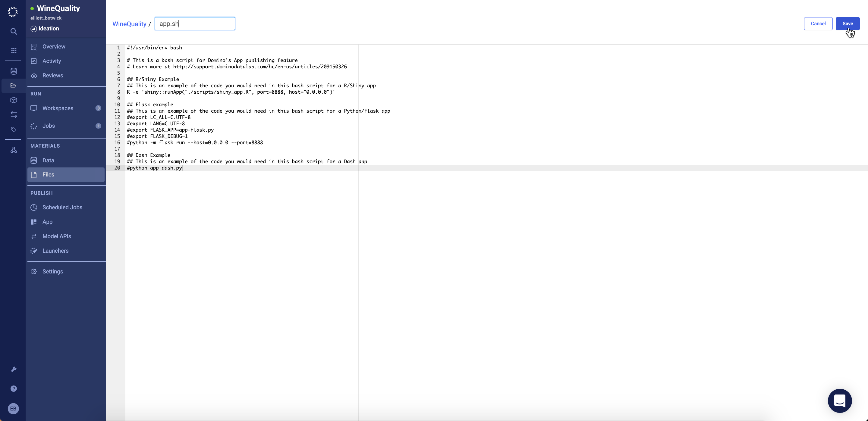
We will create a file called app.sh. It's a bash script that will start and run the Shiny App server based on the inputs provided. Copy the following code snippet.

#!/usr/bin/env bash
 
# This is a bash script for Domino's App publishing feature
# Learn more at http://support.dominodatalab.com/hc/en-us/articles/209150326
 
## R/Shiny Example
## This is an example of the code you would need in this bash script for a R/Shiny app
R -e 'shiny::runApp("./scripts/shiny_app.R", port=8888, host="0.0.0.0")'
 
## Flask example
## This is an example of the code you would need in this bash script for a Python/Flask app
#export LC_ALL=C.UTF-8
#export LANG=C.UTF-8
#export FLASK_APP=app-flask.py
#export FLASK_DEBUG=1
#python -m flask run --host=0.0.0.0 --port=8888
 
## Dash Example
## This is an example of the code you would need in this bash script for a Dash app
#python app-dash.py

Name the file app.sh and click Save.

Now navigate back into the Files tab, and enter the scripts/ folder. Click Add a new file and name it shiny_app.R (make sure the file name is exactly that, as it is case sensitive) and then paste the following into the file.

#
# This is a Shiny web application. You can run the application by clicking
# the 'Run App' button above.
#
# Find out more about building applications with Shiny here:
#
#    http://shiny.rstudio.com/
#
 
install.packages("png")
 
library(shiny)
library(png)
library(httr)
library(jsonlite)
library(plotly)
library(ggplot2)


# Define UI for application that draws a histogram
ui <- fluidPage(
  
  # Application title
  titlePanel("Wine Quality Prediction"),
  
  # Sidebar with a slider input for number of bins 
  sidebarLayout(
    sidebarPanel(
      numericInput(inputId="feat1",
                   label='density', 
                   value=0.99),
      numericInput(inputId="feat2",
                   label='volatile_acidity', 
                   value=0.25),
      numericInput(inputId="feat3",
                   label='chlorides', 
                   value=0.05),
      numericInput(inputId="feat4",
                   label='is_red', 
                   value=1),
      numericInput(inputId="feat5",
                   label='alcohol', 
                   value=10),
      actionButton("predict", "Predict")
    ),
    
    # Show a plot of the generated distribution
    mainPanel(
      tabsetPanel(id = "inTabset", type = "tabs",
                  
                  tabPanel(title="Prediction",value = "pnlPredict",
                           plotlyOutput("plot"),
                           verbatimTextOutput("summary"),
                           verbatimTextOutput("version"),
                           verbatimTextOutput("reponsetime"))
      )        
    )
  )
)
 
prediction <- function(inpFeat1,inpFeat2,inpFeat3,inpFeat4,inpFeat5) {

#### COPY FULL LINES 4-7 from R tab in Model APIS page over this line of code. (It's a simple copy and paste) ####
    
    body=toJSON(list(data=list(density = inpFeat1, 
                               volatile_acidity = inpFeat2,
                               chlorides = inpFeat3,
                               is_red = inpFeat4,
                               alcohol = inpFeat5)), auto_unbox = TRUE),
    content_type("application/json")
  )
  
  str(content(response))
  
  result <- content(response)
}
 
gauge <- function(pos,breaks=c(0,2.5,5,7.5, 10)) {
 
  get.poly <- function(a,b,r1=0.5,r2=1.0) {
    th.start <- pi*(1-a/10)
    th.end   <- pi*(1-b/10)
    th       <- seq(th.start,th.end,length=10)
    x        <- c(r1*cos(th),rev(r2*cos(th)))
    y        <- c(r1*sin(th),rev(r2*sin(th)))
    return(data.frame(x,y))
  }
  ggplot()+
    geom_polygon(data=get.poly(breaks[1],breaks[2]),aes(x,y),fill="red")+
    geom_polygon(data=get.poly(breaks[2],breaks[3]),aes(x,y),fill="gold")+
    geom_polygon(data=get.poly(breaks[3],breaks[4]),aes(x,y),fill="orange")+
    geom_polygon(data=get.poly(breaks[4],breaks[5]),aes(x,y),fill="forestgreen")+
    geom_polygon(data=get.poly(pos-0.2,pos+0.2,0.2),aes(x,y))+
    geom_text(data=as.data.frame(breaks), size=5, fontface="bold", vjust=0,
              aes(x=1.1*cos(pi*(1-breaks/10)),y=1.1*sin(pi*(1-breaks/10)),label=paste0(breaks)))+
    annotate("text",x=0,y=0,label=paste0(pos, " Points"),vjust=0,size=8,fontface="bold")+
    coord_fixed()+
    theme_bw()+
    theme(axis.text=element_blank(),
          axis.title=element_blank(),
          axis.ticks=element_blank(),
          panel.grid=element_blank(),
          panel.border=element_blank())
}
 
# Define server logic required to draw a histogram
server <- function(input, output,session) {
  
  observeEvent(input$predict, {
    updateTabsetPanel(session, "inTabset",
                      selected = paste0("pnlPredict", input$controller)
    )
    print(input)
    result <- prediction(input$feat1, input$feat2, input$feat3, input$feat4, input$feat5)
    print(result)
    
    pred <- result$result[[1]][[1]]
    modelVersion <- result$release$model_version_number
    responseTime <- result$model_time_in_ms
    output$summary <- renderText({paste0("Wine Quality estimate is ", round(pred,2))})
    output$version <- renderText({paste0("Model version used for scoring : ", modelVersion)})
    output$reponsetime <- renderText({paste0("Model response time : ", responseTime, " ms")})
    output$plot <- renderPlotly({
      gauge(round(pred,2))
    })
  })
  
}
 
# Run the application 
shinyApp(ui = ui, server = server)

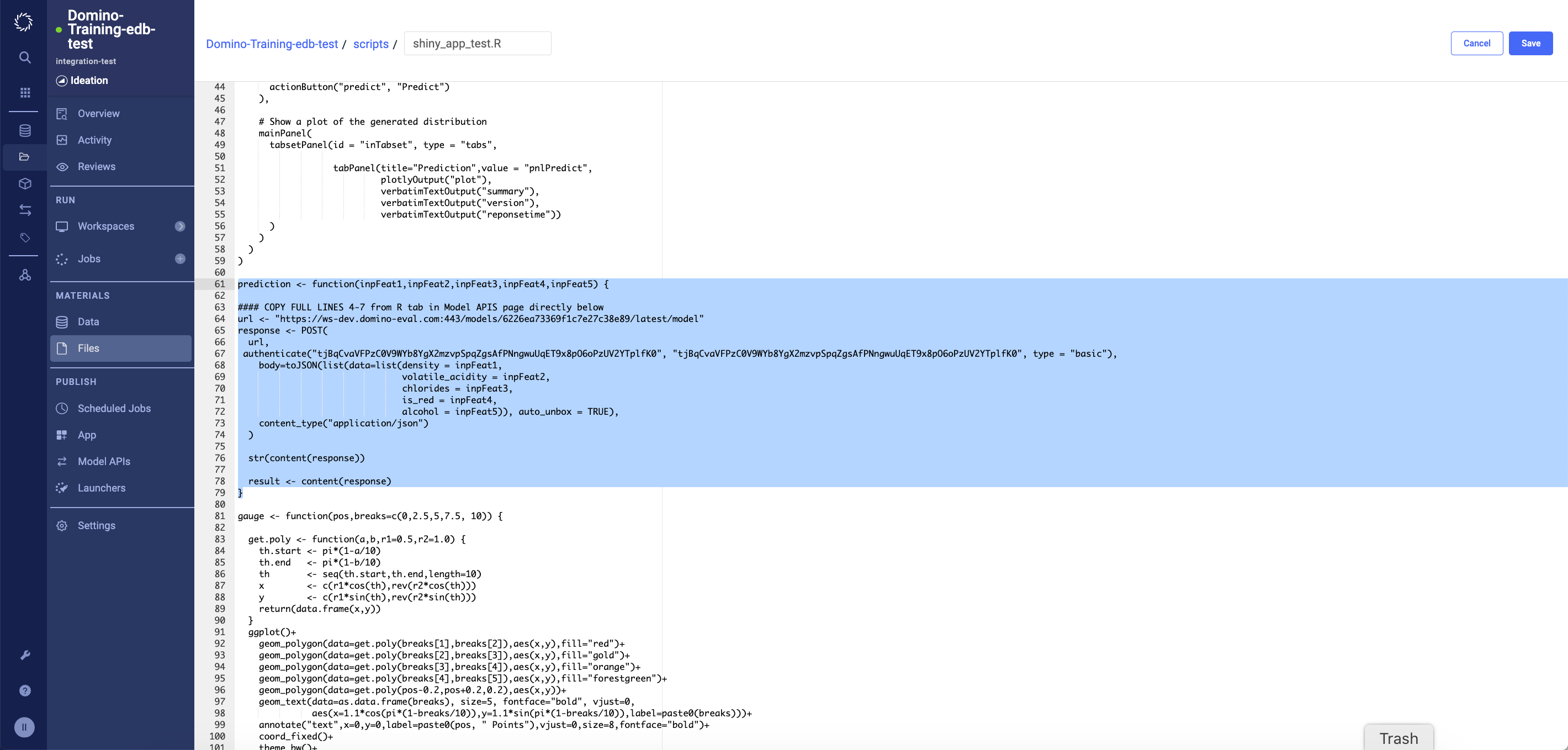
Go to line 63 note that this is missing input for your model api endpoint. In a new tab navigate to your Model API you just deployed. Go into overview and select the R tab as shown below. Copy lines 4-7 from the R code snippet. Switch back to your new file tab and paste the new lines in line 64 in your file.

Lines 61-79 in your file should look like the following (note the url and authenticate values will be different)

Click Save.

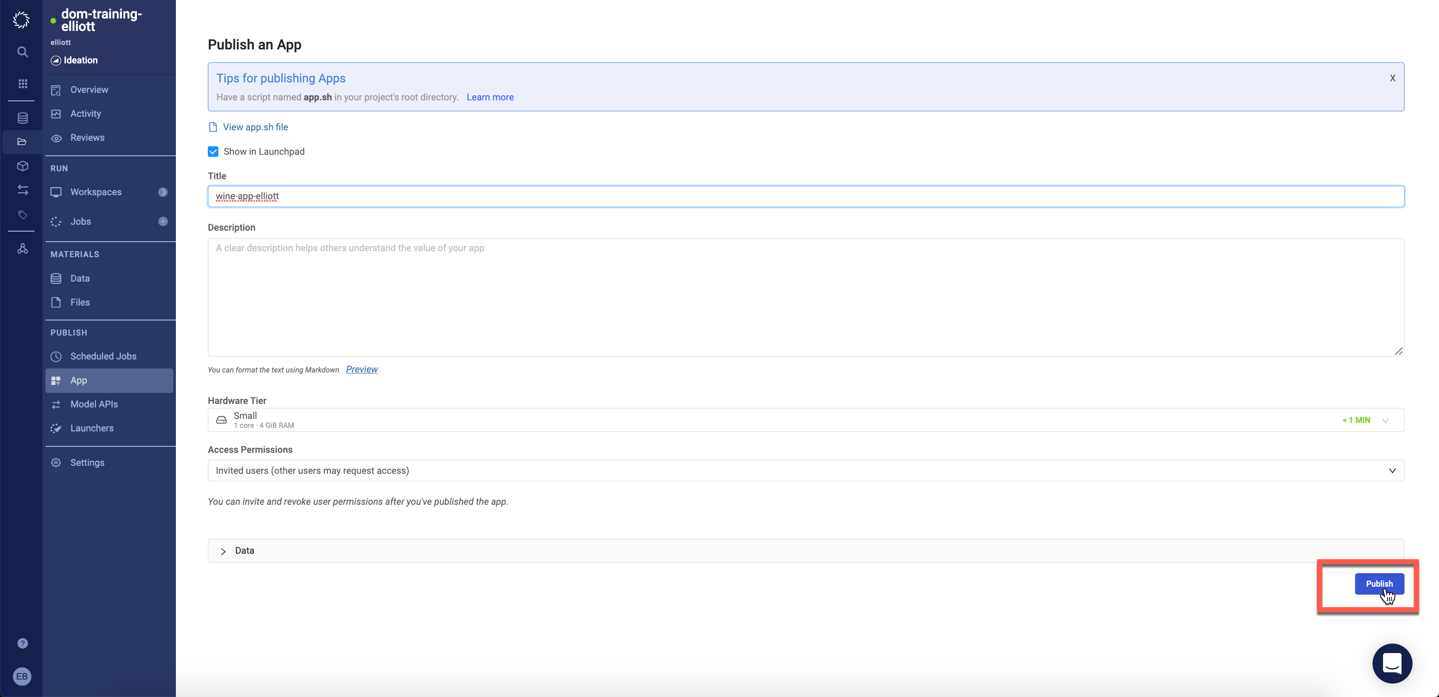
Now that you have your app.sh and shiny_app.R files created. Navigate to the App tab in your project

Enter a title for your app, e.g. 'wine-quality-yourname'

Click Publish.

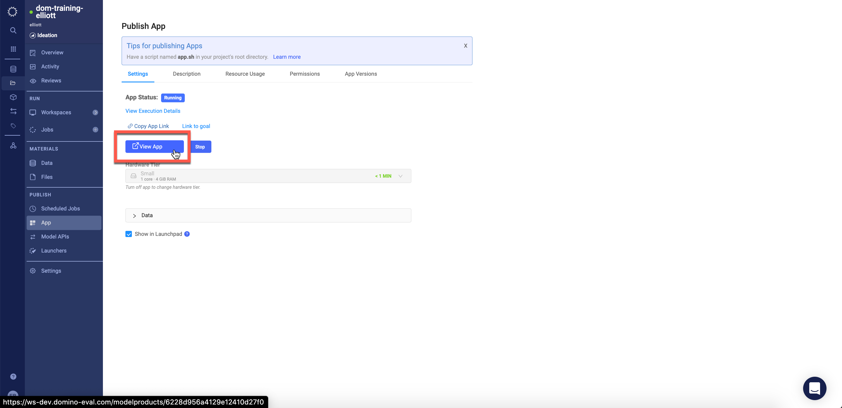
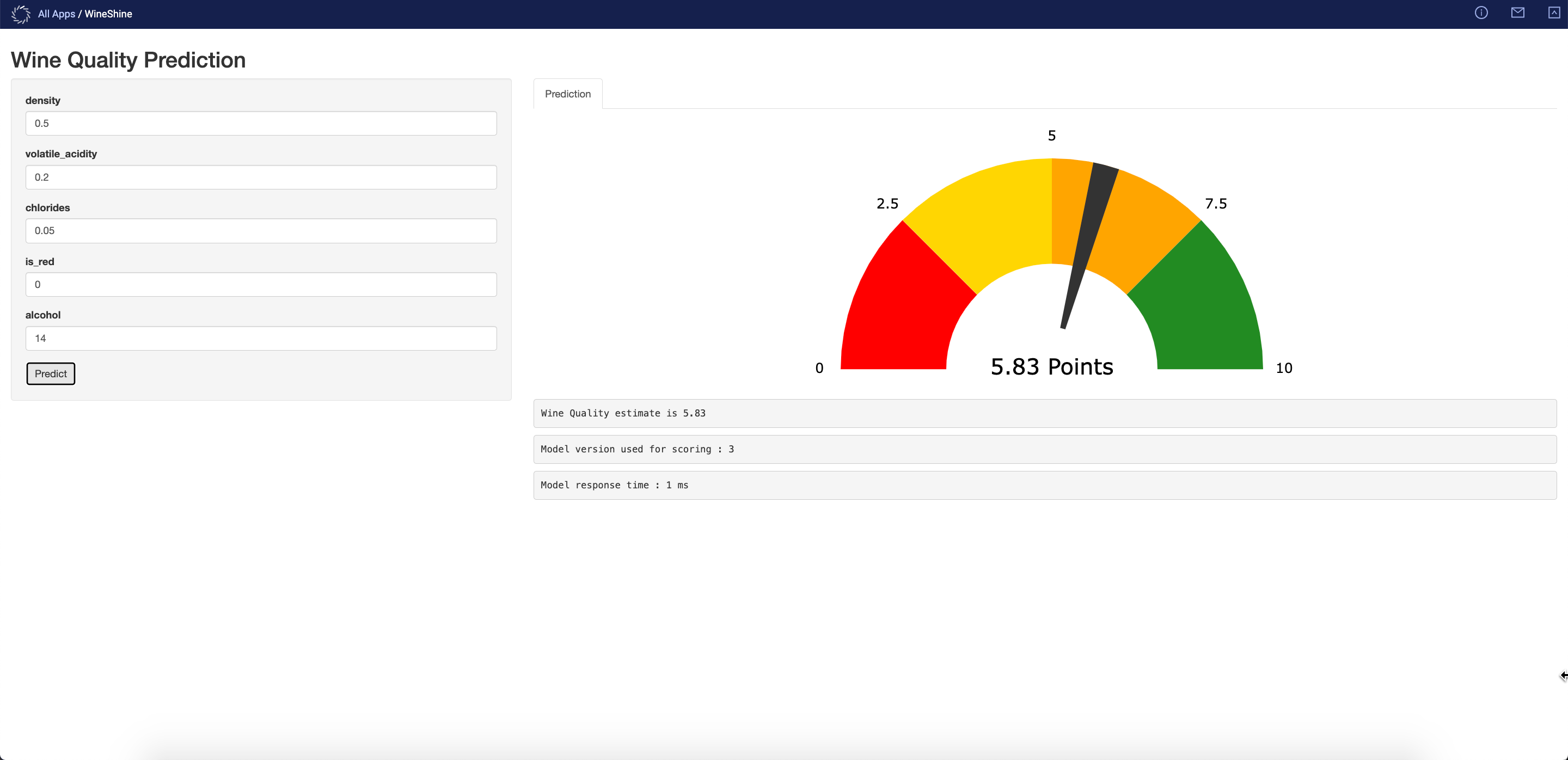
You'll now see the below screen, once your app is active (typically within ~1-3 minutes) you can click the View App button.

Try sending different scoring requests to your model using the form on the right side of your app. Click Predict to send a scoring request and view the results in the visualization on the left side.

Section 4 - Collaborate Results

Lab 4.1 - Share Web App and Model API

Congratulations! You have now gone through a full workflow to pull data from an S3 bucket, clean and visualize the data, train several models across different frameworks, deploy the best performing model, and use a web app frontend for easy scoring of your model. Now the final step is to get your model and app into the hands of the end users.

To do so we will navigate back to our project and click on the App tab

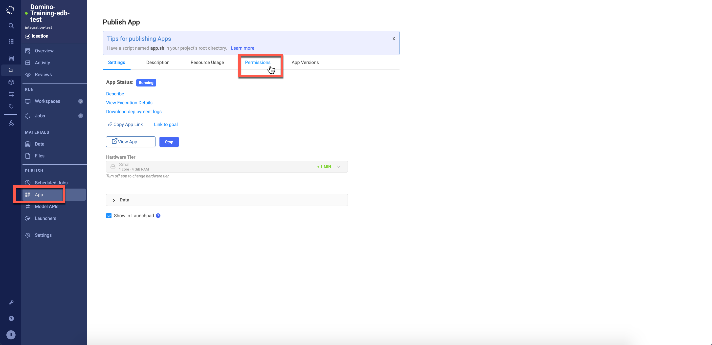
From the App page navigate to the Permissions tab

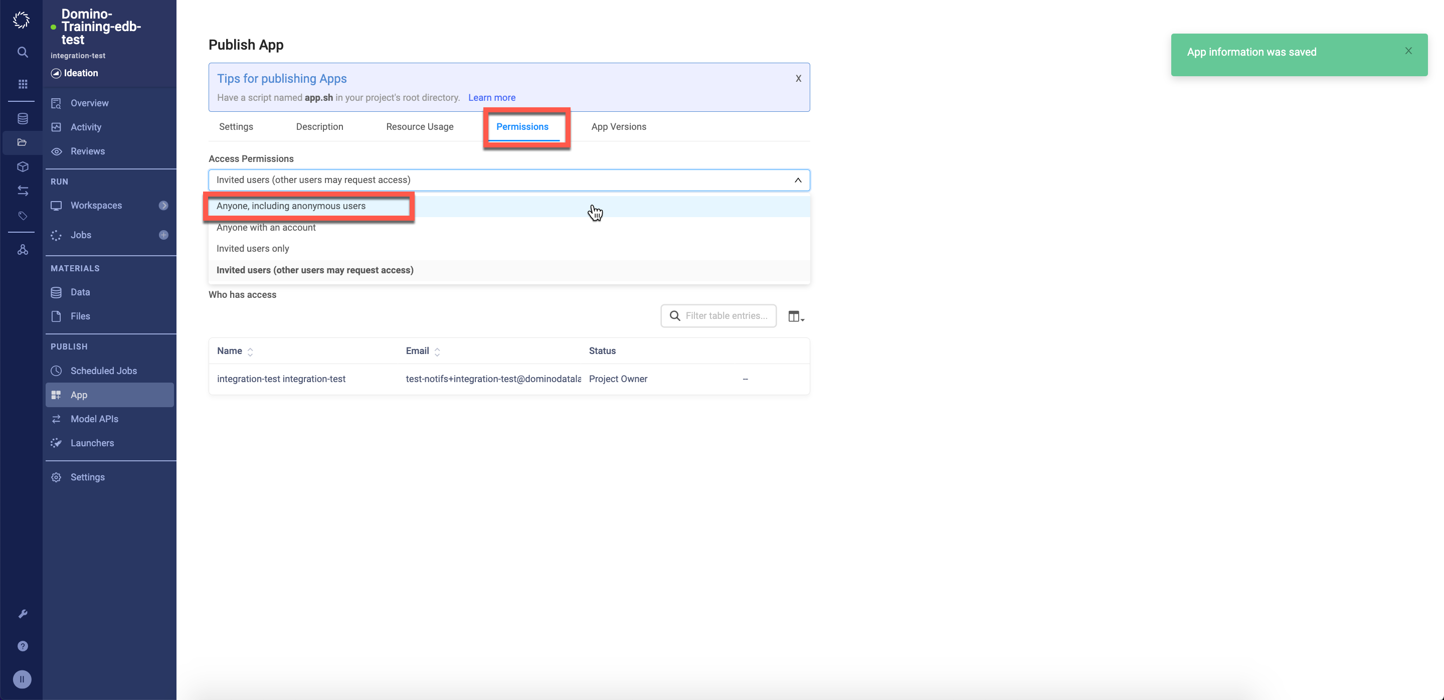
In the permissions tab update the permissions to allow anyone, including anonymous users

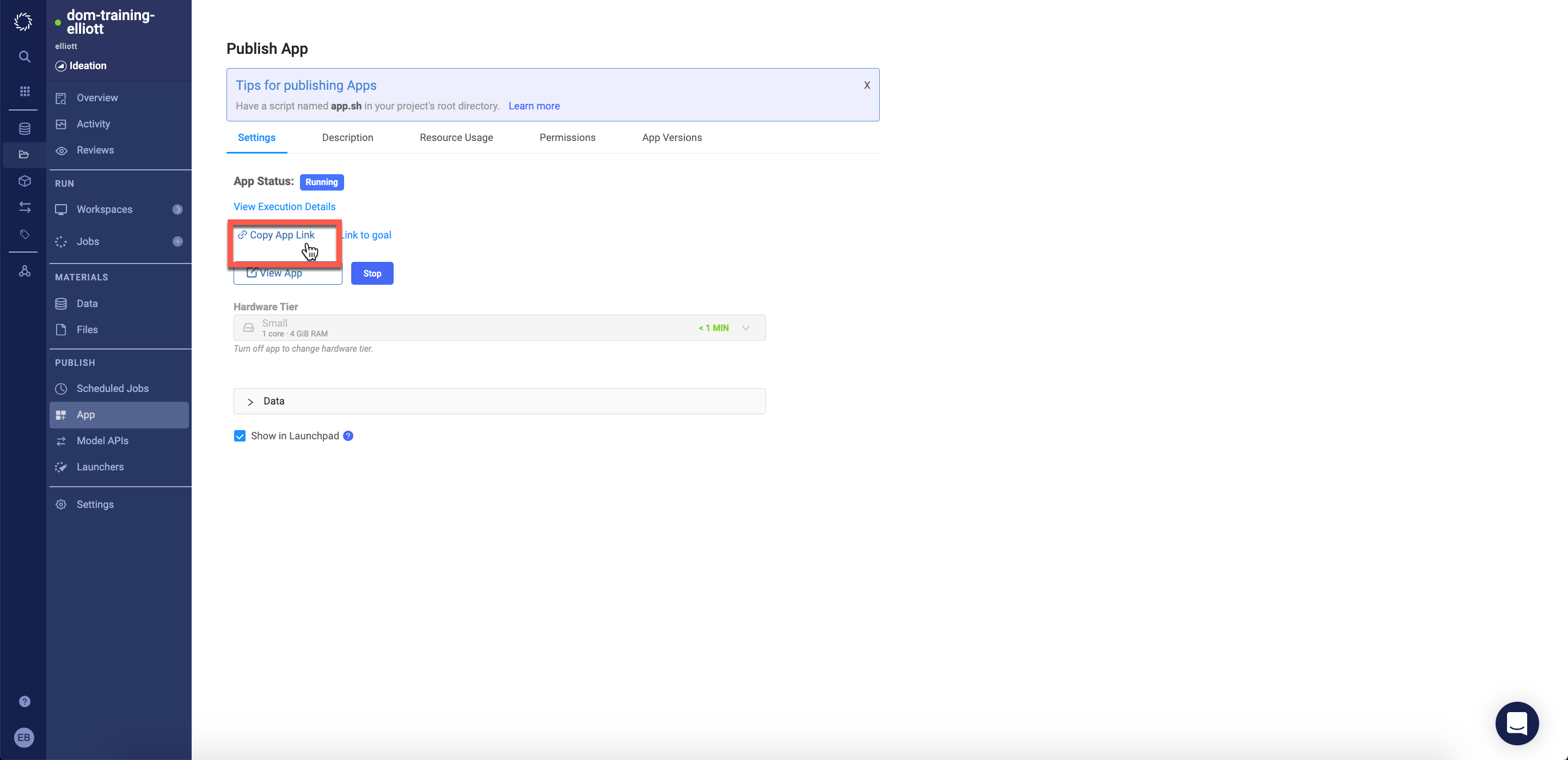
Navigate back to the Settings tab and click Copy Link to App.

With this link you're able to view the app without being logged into Domino (though you will still need to be logged into Launchpad as this trial environment blocks all other ingress).

PS - Domino provides free licenses for business users to login and view models/apps etc.

jmineroff / Domino-Launchpad-Quickstart