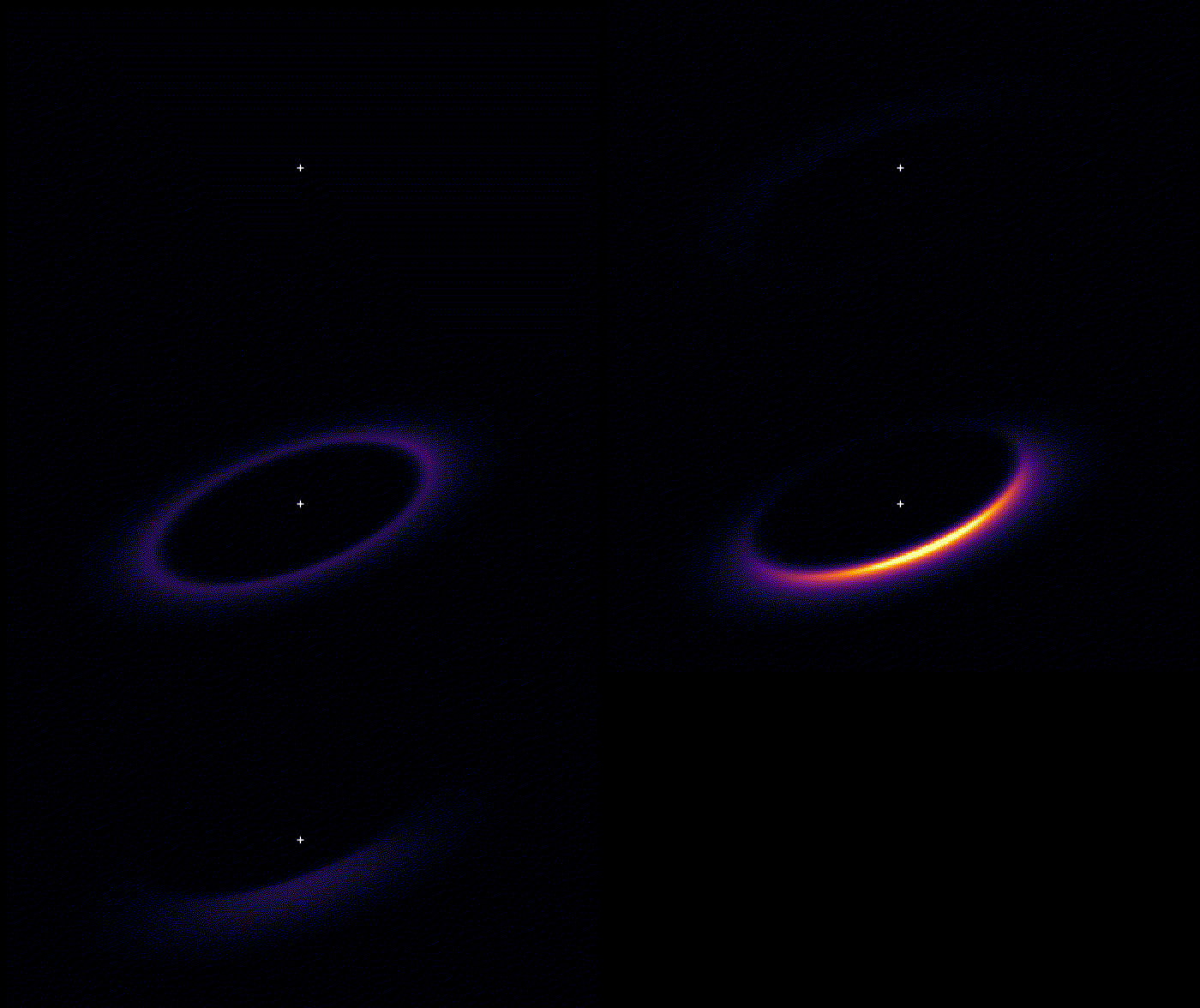
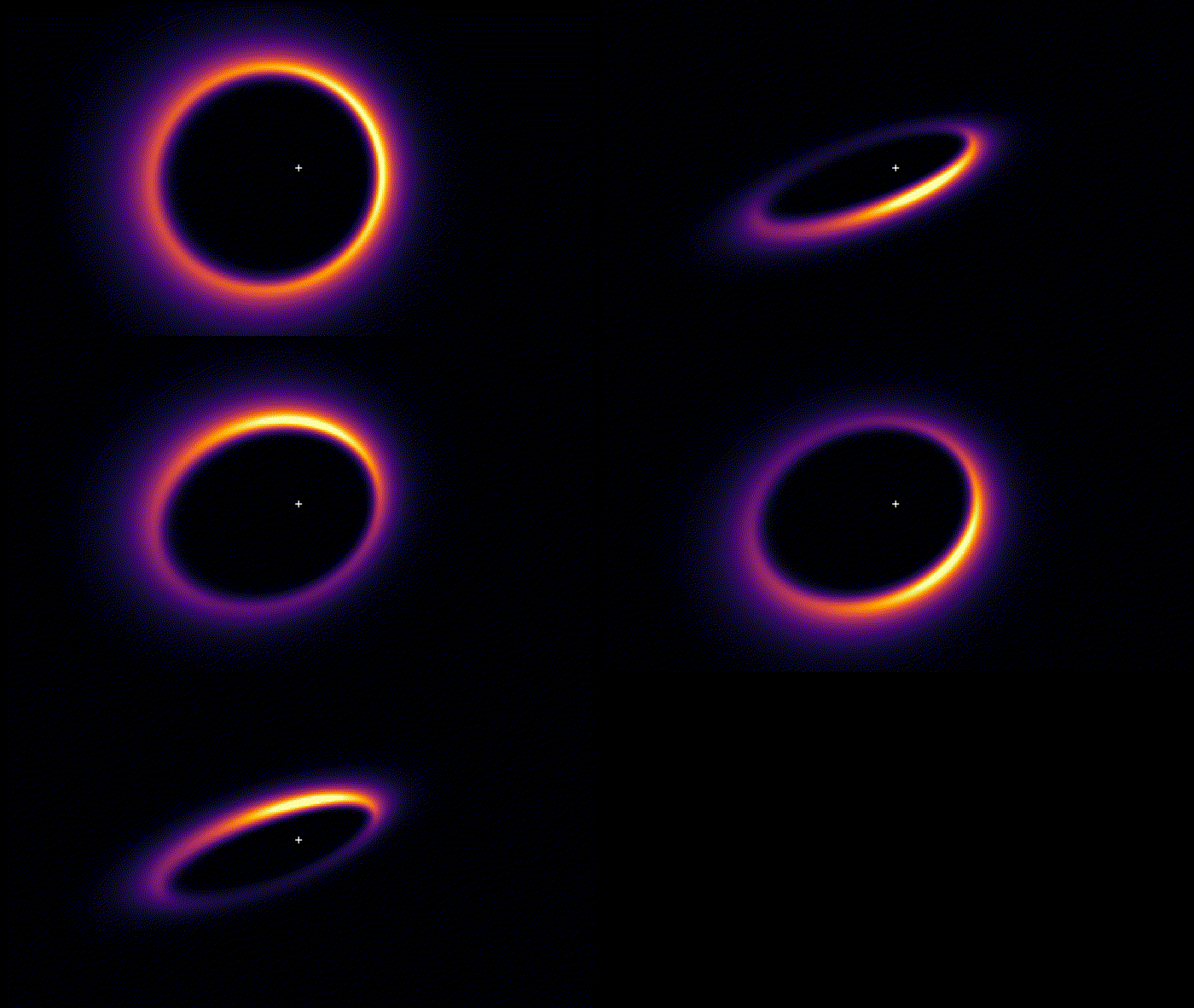
A Python code to (quickly) produce synthetic images of debris disks, either in total and polarized intensity using the Henyey-Greenstein approximation or in thermal emission (making some approximations). In the model, the disk is not infinitely flat and it should work for any inclinations except for i=0 or i=90 (otherwise there may be some division by zero).
To use the module, download the python files above and install it with the following (using the develop option so that any further changes are automatically included):
python3 setup.py developGiven that the code only uses matplotlib and numpy, it should work with python2 and python3. To compute a model, you can have a look at the end of the "DDiT.py" file, but in a nutshell, it is as simple as
from DDiT import Disk
disk = Disk()
disk.compute_model(a = 0.6, incl = 60., e = 0.3)
disk.plot()
Alternatively, if you do not want to pass the arguments to the function (let's say you want to do some MCMC and want some liberty in choosing the free parameters), you can also do the following:
from DDiT import Disk
disk = Disk()
disk.a = 0.6                 # in units of arcseconds
disk.incl = 60. * np.pi / 180.  # if defined from outside the method, has to be in radians
disk.e = 0.3
disk.compute_model()
But in that case, you have to make sure that you put the angles in radians (and check the method _check_parameters to see how the position angle is defined). Once the model is computed, you will find the images in the variables disk.intensity and disk.polarized for the total and polarized intensity. Furthermore, in disk.scattering, disk.distance, and disk.azimuth you will have access to the scattering angle, the distance to the star, and the azimuthal angle, in the midplane.
The way the code works is that it first finds a bounding box where most of the dust density distribution is contained. This bounding box, which is a 3D ellipse, is computed from the reference radius, the outer slope of the density distribution, and the eccentricity. Then, for each row of pixels perpendicular to the projected major axis of the disk (x axis), the y and z coordinates for the entry and exit points of the bounding box are estimated. The distance between the entry and exit points is divided in nframe images, and the 3D coordinates at the center of each cell are computed. The radial and vertical volumetric density are evaluated at the center of the grid. For scattered light or polarized intensity, the scattering angle is estimated from the 3D coordinates and the phase function is assumed to follow the Henyey-Greenstein approximation (with one coefficient for total intensity, and one coefficient for the polarized intensity). For thermal emission images, the temperature of the dust grain is computed using Eq. 3 of Wyatt 2008, Tdust = 278.3/np.sqrt(r) where r is the distance of the center of the grid to the star. Then the dust density is multiplied by a Planck function at the proper temperature. The final image is the sum of all those nframe images. The process is highlighted in the animation below.
The Disk class has three possible parameters which are the following:
nx = 300             # Size of the image in pixels
pixscale = 0.01226   # Size of one pixel in arcseconds
nframe = 50          # Number of frames (see above)
Both values of nframe and nx should be integers, and nx should be an even number. Once the class is called for the first time, those parameters should not be changed, otherwise you may get some very strange results. To compute thermal emission images, two other parameters should be provided:
thermal = True       # A boolean
dpc = 35.34          # Distance of the central star in pc
The distance is only necessary to normalize the temperature distribution as explained above. Afterwards, the method compute_model has the following input parameters:
a = 0.85             # Semi-major axis of the disk in arcseconds
incl = 60.           # Inclination, in degrees
pa = 112.            # Position angle, in degrees
pin = 5.0            # Inner slope of the density distribution (>0)
pout = -15.0         # Outer slope of the density distribution (<0)
e = 0.1              # Eccentricity
omega = 85.          # Argument of periapsis, in degrees
gsca = 0.5           # Henyey-Greenstein coefficient for total intensity
gpol = 0.5           # Henyey-Greenstein coefficient for polarized intensity
opang = 0.03         # Opening angle of the disk, in radians
s11 = None           # Scattered light phase function
s12 = None           # Polarized light phase function
Most of the parameters are self-explanatory, except the last two, which allow the user to provide arrays for the shape of the phase function, either in total or polarized intensity. The arrays should have two dimensions, so that there can be a phase function for the north and south sides of the disk. For instance, if one wants to define an isotropic polarized phase function for both sides, then s12 can be defined as np.ones(shape=(nb,2)) where nb is the number of scattering angles between 0 and 180 degrees. If either s11 or s12 is provided, the code automatically define an array disk.theta containing the scattering angles (in radians). One should note that if the user only provides s11 (or s12) the code will automatically assign an isotropic phase function for s12 (or s11).
The second dimension of the array is not necessarily always the north or south side, as it will depend on the position angle of the disk, so if you wish to use this feature you will have to make some tests to identify which side is which.
For thermal emission, the user should provide an additional parameter:
wave = 850. # Wavelength in micronsIn that case, the parameters gsca, gpol, s11, and s12 are no longer relevant (but the code will not complain).
The animation above showcases that the whole range of inclinations can be probed, and each image takes less than a few seconds to be computed. As a matter of fact, you will see that the computing time strongly depends on the inclination, because for face-on disks, there are more pixels where the dust density is not null, while for edge-on disks, the vast majority of the pixels do not intercept the bounding box of the disk. Finally, as a small note, in this animation, the scattered light phase function is slightly forward scattering (gsca = 0.4), but the disk does not become much brighter as the inclination increases because the cuts are re-evaluated for each frame.
If you use this code for your research, feel free to contact me if you have any doubt or question, and please cite the following paper:
Olofsson et al. (2020) "The challenge of measuring the phase function of debris disks. Application to HR,4796"


