jinchenglee/CarND-Advanced-Lane-Lines

##Advance Lane Finding

Highlights of this project:

Compute the camera calibration matrix and distortion coefficients given a set of chessboard images.
Apply a distortion correction to raw images.
Use color transforms, gradients, etc., to create a thresholded binary image.
Apply a perspective transform to rectify binary image ("birds-eye view").
Detect lane pixels and fit to find the lane boundary.
Determine the curvature of the lane and vehicle position with respect to center.
Warp the detected lane boundaries back onto the original image.
Output visual display of the lane boundaries and numerical estimation of lane curvature and vehicle position.

Implementation Details

###Camera Calibration

####1. Camera intrinsic matrix and distortion coefficients.

The OpenCV checkerboard calibration program is based on Professor Z. Zhang's paper "Z. Zhang. "A flexible new technique for camera calibration".".

Calibration process calculates intrinsics (camera 3D coordinates to image 2D coordinates using pinhole camera model) and extrinsics (Rotation R and Translation T from world 3D coordinates to camera 3D coordinates). Mathoworks explanation page on this.

OpenCV implementation source code can be found here. The OpenCV implementation involves non-linear optimization, such as Levenberg-Marquardt method, as it is a non-linear model, such as the distortion models.

$$\lambda \begin{bmatrix} u \\ v \\ 1 \end{bmatrix} = K_{3X3} * R_{3X4} * \begin{bmatrix} x \\ y \\ z \\ 1 \end{bmatrix} + T_{3X1}$$

The code for this step is contained in lines 18 through 71 of file camera_cal.py.

I start by preparing "object points", which will be the (x, y, z) coordinates of the chessboard corners in the world. Here I am assuming the chessboard is fixed on the (x, y) plane at z=0, such that the object points are the same for each calibration image. Thus, objp is just a replicated array of coordinates, and objpoints will be appended with a copy of it every time I successfully detect all chessboard corners in a test image. imgpoints will be appended with the (x, y) pixel position of each of the corners in the image plane with each successful chessboard detection.

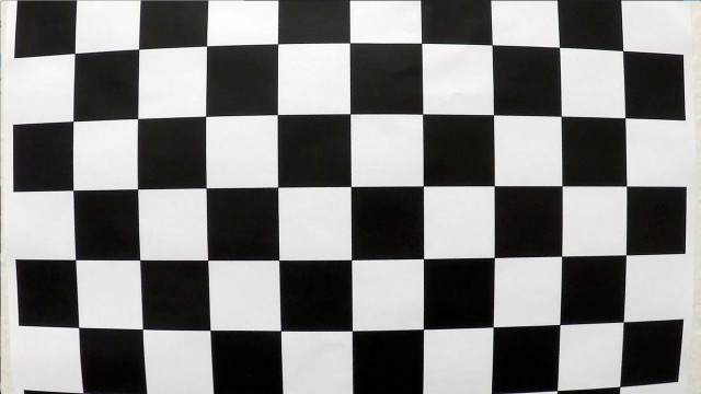
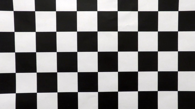
I then used the output objpoints and imgpoints to compute the camera calibration and distortion coefficients using the cv2.calibrateCamera() function. I applied this distortion correction to the test image using the cv2.undistort() function and obtained this result.

Original image:

Undistorted image:

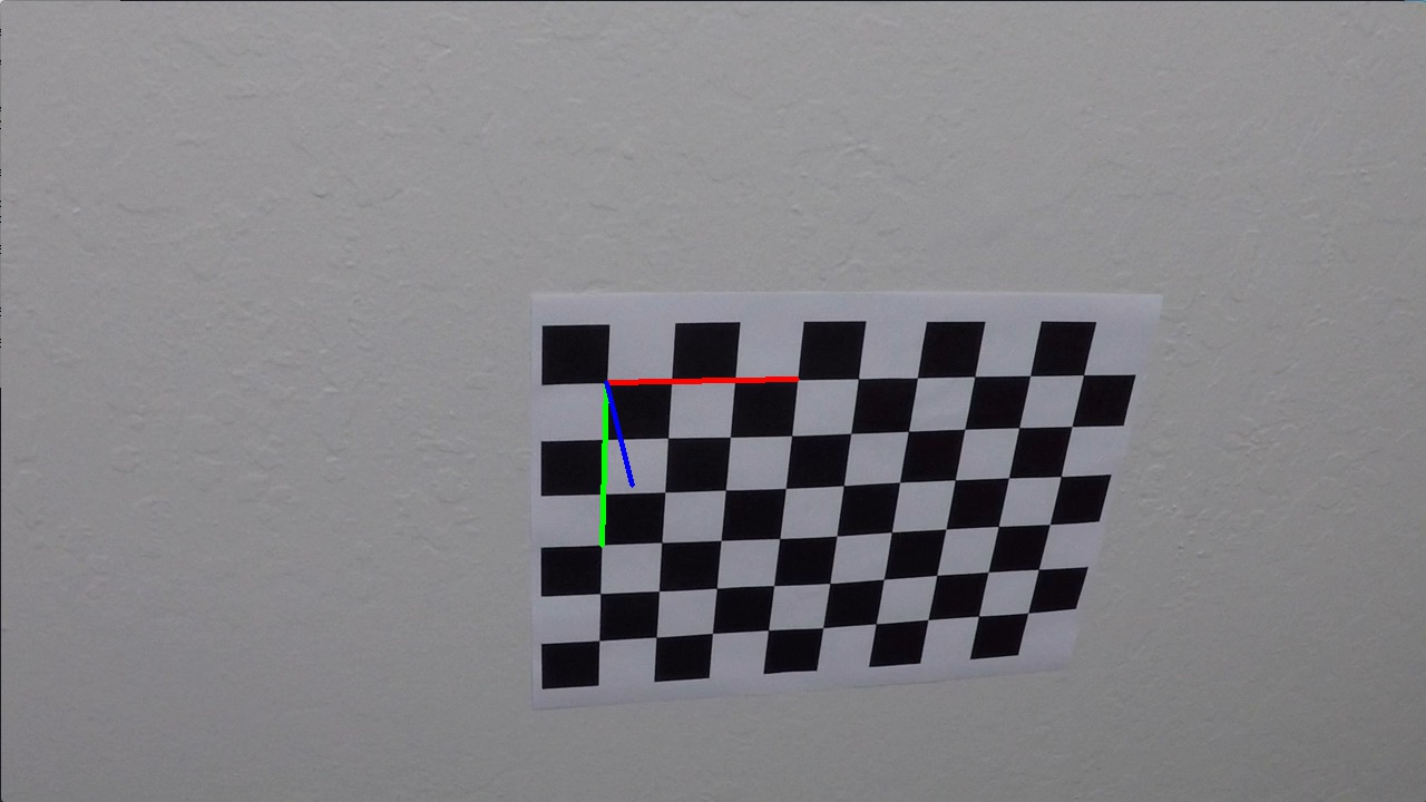
Draw the "world coordinates axises" on one of the checkerboard image.

	...
	# OpenCV API returns:
	#  mtx (intrinsic matrix), dist (distortion parameters), 
	#  rvecs (Rodriguez vector), tvecs (Translation vector)
	ret, mtx, dist, rvecs, tvecs = cv2.calibrateCamera(objpoints, imgpoints, img_size,None,None)
	...
	
	# --------------------
	# World co-ordinates of axis points
	# --------------------
	objp = np.array([
    	[0.,0.,0.], # Origin
    	[3.,0.,0.], # X (red axis)
    	[0.,3.,0.], # Y (green axis)
    	[0.,0.,-3.] # -Z (blue axis)
	])

	# Project above points to a specific image
	image_pt, _ = cv2.projectPoints(objp, rvecs[0], tvecs[0], mtx, dist)

Axises are lines connecting above points. Please be noticed the Z axis is negative. Also, the abosolute dimension is missing here, which is unnecessary to derive camera intrinsic and extrinsic matrices in calibration process for mono-camera using Zhang's method.

###Pipeline (single images)

####1. Distortion-corrected image Loading previously saved parameters in pickle file when I did camera calibration using checkerboard, I used OpenCV API undistort to do image distortion-correction before any further processing as below.

# Undistort
f = open('camera_cal/wide_dist_pickle.p', 'rb')
param = pickle.load(f)
K = param["mtx"]        # Camera intrinsic matrix
d = param["dist"]       # Distortion parameters
image = cv2.undistort(image, K, d, None, K)
mpimg.imsave("test_images/test1_undistorted.png", image)

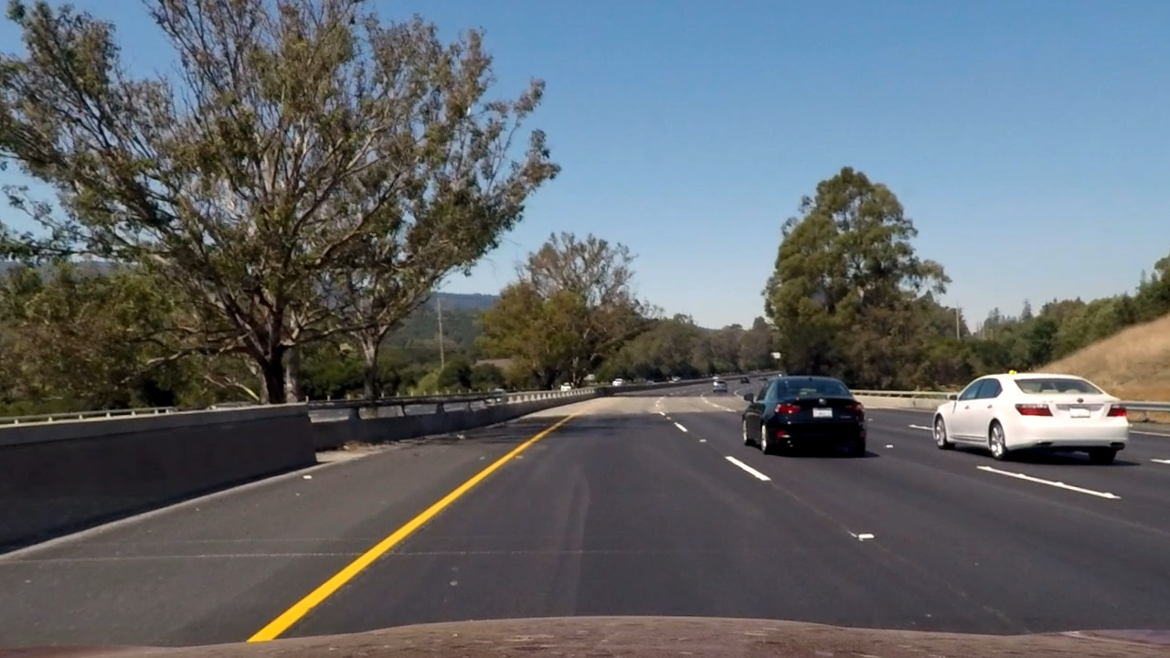
The distortion-corrected image example:

####2. Thresholded binary image

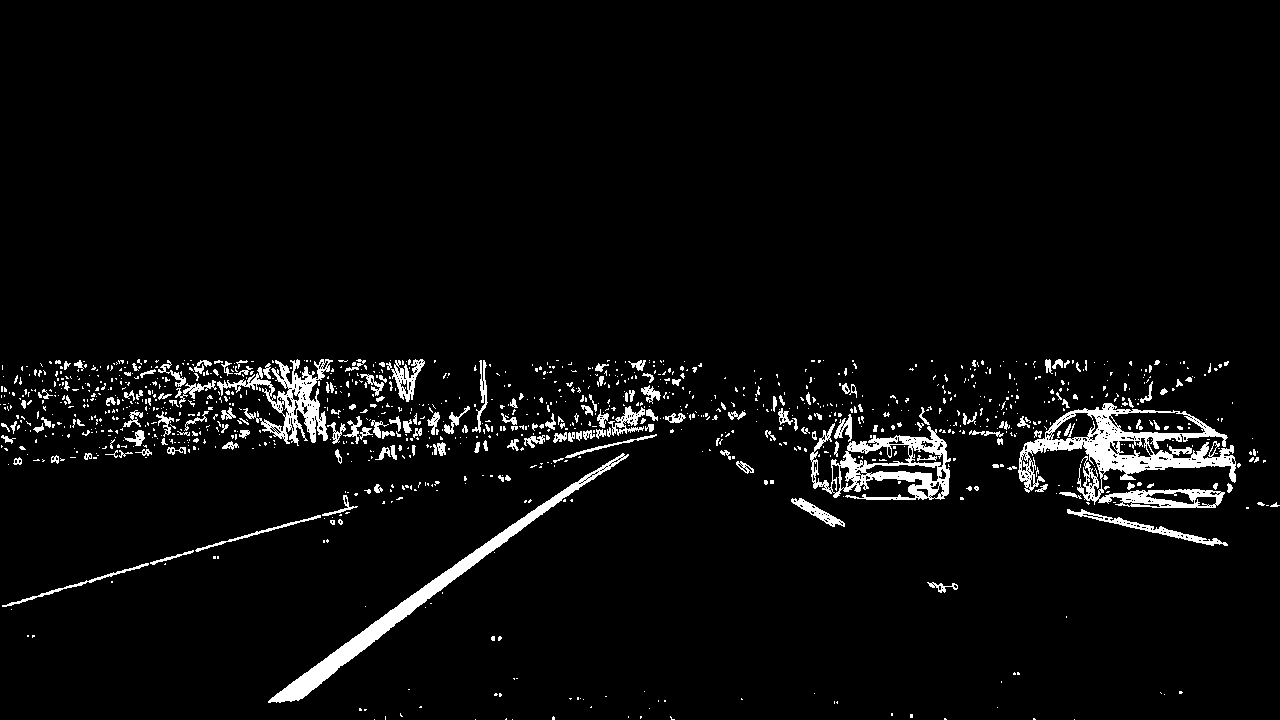
I used a combination of AOI (area of interest), color and gradient thresholds to generate a binary image. Here's an example of my output for this step. (note: this is not actually from one of the test images)

    # Convert to HSV color space and separate the V channel
    hsv = cv2.cvtColor(img, cv2.COLOR_RGB2HLS).astype(np.float)

    # AOI (area of interest) mask - we only care about lower part of the image
    size_x, size_y, size_ch = hsv.shape
    hsv[0:size_x//2,:,:] = 0
    l_channel = hsv[:,:,1]
    s_channel = hsv[:,:,2]

    # Sobel x on L channel
    sobelx = cv2.Sobel(l_channel, cv2.CV_64F, 1, 0, ksize=sobel_ksize) # Take the derivative in x
    abs_sobelx = np.absolute(sobelx) # Absolute x derivative to accentuate lines away from horizontal
    scaled_sobel = np.uint8(255*abs_sobelx/np.max(abs_sobelx))

    # Threshold x gradient
    sxbinary = np.zeros_like(scaled_sobel)
    sxbinary[(scaled_sobel >= sx_thresh[0]) & (scaled_sobel <= sx_thresh[1])] = 1

    # Threshold Saturation color channel
    s_binary = np.zeros_like(s_channel)
    scaled_s_ch = np.uint8(255*s_channel/np.max(s_channel))
    s_binary[(scaled_s_ch >= s_thresh[0]) & (scaled_s_ch <= s_thresh[1])] = 1

    # Combine the output - OR the two selections.
    binary = np.zeros_like(s_channel)
    binary[(sxbinary==1) | (s_binary==1)] = 1

####3. Perspective transform for Birds-Eye-View

The code for my perspective transform includes a function called warper(), which appears in top lines in the file perspective.py. The warper() function takes as inputs an image (img), as well as source (src) and destination (dst) points. I chose the hardcode the source and destination points in the following manner:

src = np.float32(
    [[(img_size[0] / 2) - 65, img_size[1] / 2 + 100],
    [((img_size[0] / 6) - 10), img_size[1]],
    [(img_size[0] * 5 / 6) + 60, img_size[1]],
    [(img_size[0] / 2 + 65), img_size[1] / 2 + 100]])
dst = np.float32(
    [[(img_size[0] / 4), 0],
    [(img_size[0] / 4), img_size[1]],
    [(img_size[0] * 3 / 4), img_size[1]],
    [(img_size[0] * 3 / 4), 0]])
...
    # Get the perspective change matrix
    M = cv2.getPerspectiveTransform(src, dst)
    # Apply the perspective change
    warped_img = cv2.warpPerspective(img, M, img_size, flags=cv2.INTER_NEAREST)  # keep same size as input image

This resulted in the following source and destination points:

Source	Destination
575, 460	320, 0
203, 720	320, 720
1127, 720	960, 720
705, 460	960, 0

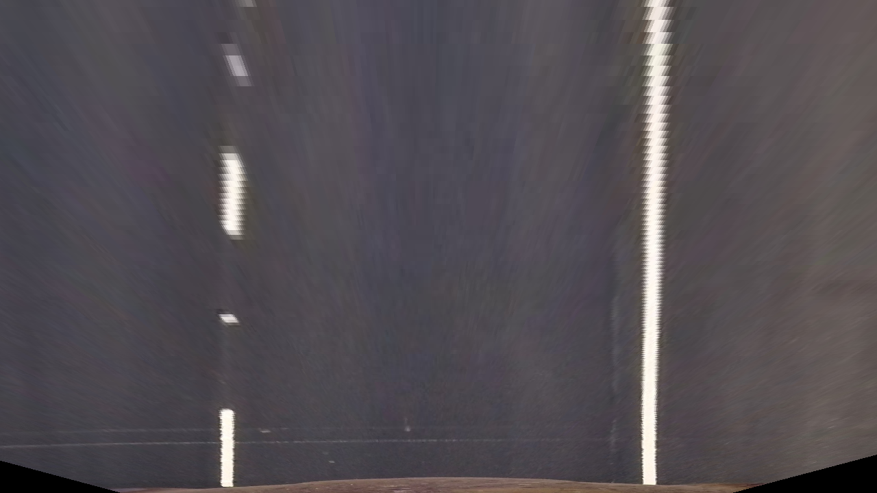
I verified that my perspective transform was working as expected by drawing the src and dst points onto a test image and its warped counterpart to verify that the lines appear parallel in the warped image.

Verified on another sample image after warping:

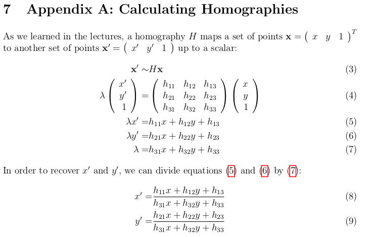
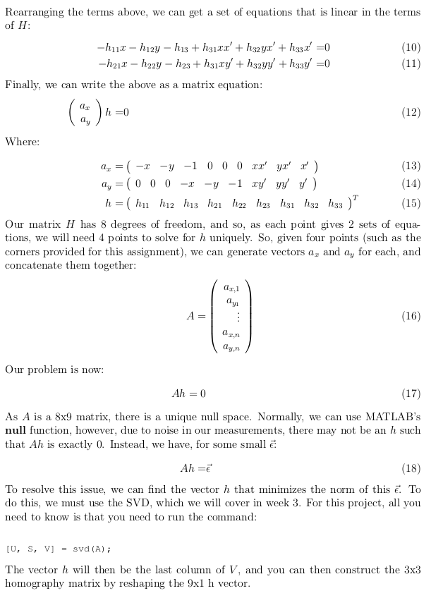
Theory behind the perspective transform matrix can be found from Coursera course Robotics Perception by Univ. Pensyvania, week2 assignment notes.

####4. Lane-line detection using polynomial

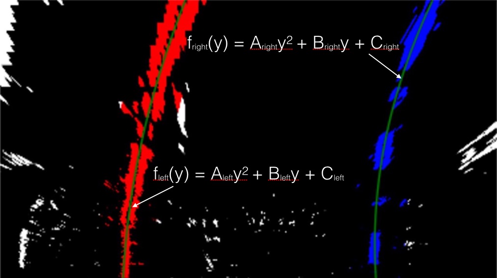
Then I did some other stuff and fit my lane lines with a 2nd order polynomial kinda like this in lane_detector.py:

It starts with histogram of image columns. the left/right lane pixels should have histogram peaks in left and right side if searching from mid-point.

    # Take a histogram of the bottom half of the image
    histogram = np.sum(binary_warped[binary_warped.shape[0]//2:,:], axis=0)

    # Find the peak of the left and right halves of the histogram
    # These will be the starting point for the left and right lines
    midpoint = np.int(histogram.shape[0]/2)
    leftx_base = np.argmax(histogram[:midpoint])
    rightx_base = np.argmax(histogram[midpoint:]) + midpoint

The peaks are set to be starting base points of left/right lanes.

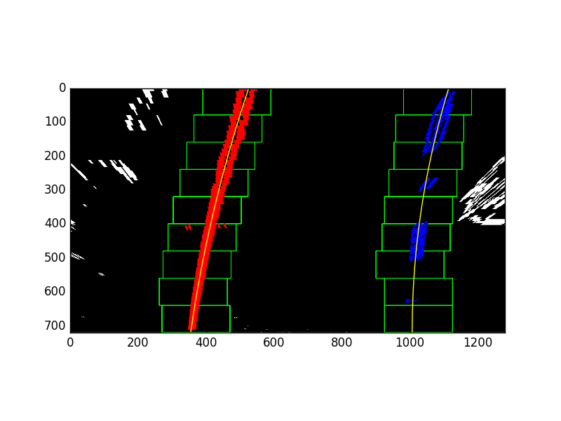
Then a window searching approach is taken to gradually search upwards from the left/right base point to find points clustered right above. These newly found points are meaned to find new base points for next round of window search upwards. There are a total of 9 layers of windows as below.

All the lane line pixels are saved for polynominal fit calculation.

    # Extract left and right line pixel positions
    leftx = nonzerox[left_lane_inds]
    lefty = nonzeroy[left_lane_inds]
    rightx = nonzerox[right_lane_inds]
    righty = nonzeroy[right_lane_inds]

    # Fit a second order polynomial to each
    left_fit = np.polyfit(lefty, leftx, 2)
    right_fit = np.polyfit(righty, rightx, 2)

The left_fit/right_fit values (shape=[1,3]) are updated for each input frame image. Except for the very 1st frame when left_fit/right_fit don't exist, all follow up frames can do "smarter" window search along previous frame fit curve.

####5. Radius of curvature of the lane and the position of the vehicle with respect to center

The detected lane is fit to a 2nd order polynomial curve $$f(y)=Ay^2+By+C$$.

As a result, the radius of curvature is calculated using:

$$R_{curve} = {(1+(2Ay+B)^2)^{3/2} \over |2A|}$$

As to the car position, it is calculated using 640 minus midpoint of bottom-most left lane and right lane position in pixel values, then scale it to meters. This works under the assumption that the camera is mounted right at the middle of the car. When the car is right at the middle of the lane, the average of left/right lane position in pixel should be half of image width, 640.

I did these in function cal_curvature in my code in lane.py:

    def cal_curvature(self, binary_warped):
        # Measure curvature

        left_fit = self.cur_l_fit
        right_fit = self.cur_r_fit

        ym_per_pix = 30/720 # Assuming 30 meters per pixel in y dimenstion
        xm_per_pix = 3.7/700 # 3.7 meters per pixel in x dimenstion

        ploty = np.linspace(0, binary_warped.shape[0]-1, binary_warped.shape[0] )
        leftx= left_fit[0]*ploty**2 + left_fit[1]*ploty + left_fit[2]

        y_eval = np.max(ploty) # Select the bottom line position to evaluate
        # Fit new polynomials to x,y in world space
        left_fit_cr = np.polyfit(ploty*ym_per_pix, leftx*xm_per_pix, 2)
        # Calculate the new radii of curvature
        left_curverad = ((1 + (2*left_fit_cr[0]*y_eval*ym_per_pix + left_fit_cr[1])**2)**1.5) / np.absolute(2*left_fit_cr[0])
        # Now our radius of curvature is in meters
        #print(left_curverad, 'm')

        # Find car position as to center of lane
        leftx= left_fit[0]*y_eval**2 + left_fit[1]*y_eval + left_fit[2]
        rightx= right_fit[0]*y_eval**2 + right_fit[1]*y_eval + right_fit[2]
	
	# Assuming camera is mounted at center of the car.
	# Negative means in left part of the lane.
        off_x = 640 - (leftx + rightx)//2
        off_center = off_x * xm_per_pix

####6. Example image of your result plotted back down onto the road such that the lane area is identified clearly.

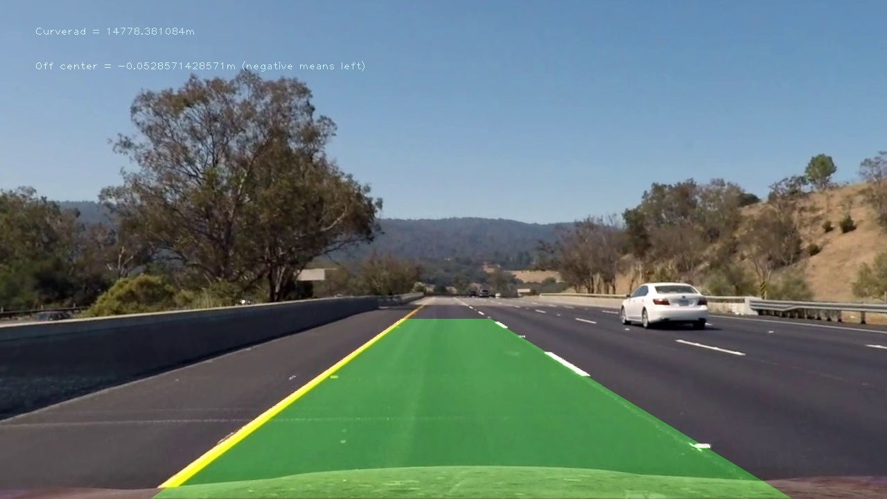
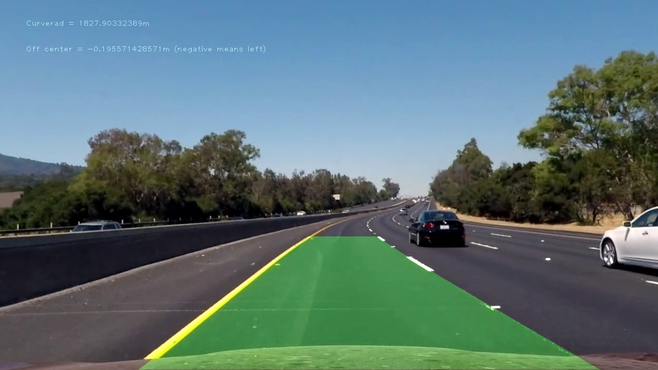
I implemented this step in function draw_lane_area() in my code in lane.py. Here is a few examples of my result on a test image:

###Pipeline (video)

####1. Final video output.

Here's a link to my video result

###Discussion

####1. Problems / issues and TODO list

Current implementation failed with both challenge videos. These are the challenges:

Several vertical edges sit close to each other (such as in challenge_video.mp4), which easily confuses the searching window. This has to be resolved using better binary filter technique, probably adaptive ones.
Brightness and light reflection sensitive. In harder_challenge_video.mp4, there are cases input video image suddenly becomes much brighter that filtering binary, with fixed threshold, cannot differentiate features. Again, adaptive filtering threshold and/or input image histogram equalization should both help.

jinchenglee / CarND-Advanced-Lane-Lines

Implementation Details

About

Languages