Tuna Prediction

^{Predicting the location of Tuna 🐟 using SVM (Support Vector Machine) through Python and Dash.}

Introduction

The initial goal of our program is to predict tuna location based on fishing vessel data and its correlation with sea surface temperature (SST) and chlorophyll concentration. We also want to see the comparison of different prediction model performance. Why we predict tuna location using fishing vessel data? because every fishing vessel in this data has fishing gear capable to fish tuna, so we assume they fish tuna. Why sea surface temperature and chlorophyll concentration become predictor for predicting tuna location? because tuna lives in certain sea surface temperature and tuna eat small fish and invertebrates that eat plankton in certain chlorophyll concentration.

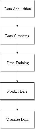
Because of that, we need to acquire fishing vessel data, chlorophyll concentration data, and sea surface temperature data. The fishing vessel data is from Global Fishing Watch, chlorophyll concentration data is from OceanWatch, and sea surface temperature data is from NOAA. The fishing vessel data has 4 attributes : latitude, longitude, geartype and fishing hours. Latitude and longitude is the coordinate of fishing vessel, geartype is type of fishing gear that fishng vessel have, and fishing hours is the duration fishng vessel stay in that position. All fishing vessel is equipped with gear that is capable to fish tuna so we can assume that they fish tuna in that coordinate. Based on value of fishing hours, we can make new attributes which is tuna. We can determine tuna value based on if fishing hours value is more than zero then tuna value is 1 and if the otherwise then tuna value is 0. We assume that tuna location is the same as fishing vessel coordinate which fishing hours is more than zero because we assume that they fish tuna in that coordinate. After we determine tuna value, we combine value from fishing vessel data, sst data, and chlorophyll concentration data. Then we make training data which consist of sst value, chlorophyll value, fishing hours, and tuna value. After we make training data, we make prediction model to predict whether in that coordinate there is tuna or not. The prediction model consists of tuna as target and sst and chlorophyll as feature. After that, we make 3 different prediction model : prediction model that use 60% data training, prediction model that use 70% data training, and prediction model that use 80% data training. After we make 3 prediction model, we predict tuna location coordinate. After predicted tuna location coordinate is obtained, we visualize predicted tuna location coordinate data from each prediction model.

Getting Started

To be able to run this app, you will need to have the following prerequesites and have to follow the instructions below.

Prerequisites

Python 3 with the following additional libraries:

pandas
dash
dash-table
dash-bootstrap-components
plotly

Running the application

Make sure you have all the prerequisites installed and you are connected to the internet. Then clone/download "CombinedUPDATED.zip", extract the folder, open terminal/cmd and navigate to the folder and run app.py:

python app.py

If all works well this is the console should show the IP address of where the dashboard is hosted.

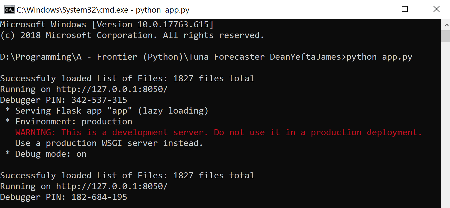
Then copy and paste the IP address to your browser in order to access the application's user interface and it should show similar to the image below.

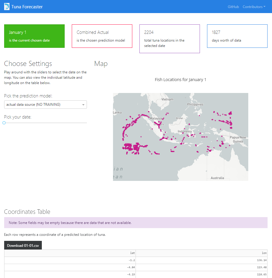
By default, the dashboard shows the "actual" data which consists of the real raw data that we have not manipulated in any way. This data is what we used to train our model on. You can change this by picking the prediction model from the dropdown menu.

You can play around with the dashboard by directly manipulating the slider to pick the date and the map and UI will change accordingly.

You can also play around with the interactive map by zooming in, picking the points you want, highlighting over the points to see the coordinates and more.

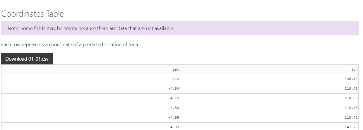
Last but not least, you can scroll down and view/download the individual coordinates of each point from the table on the bottom of the page.

Explanation

On the following sections, we will explain the techniques that we have used to achieve our results.

Data Cleansing

Before the data is trained, we had to clean the data first in order for our model to not be distorted.

tunaDataCleanerSSTChlorophyll.py

This python script is responsible for automatically iterating through the original data source folder, cleaning the data, and then saving the new cleaned data files in a new folder.

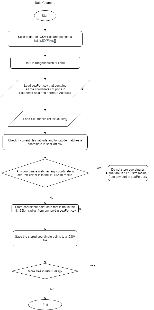
Since our data is a collection of coordinates of boats around Southeast Asia we wanted to make sure that these boats are out to fish and not parked in a sea port. Therefore, to clean the data, we had to search for the coordinates of seaports that surround Southeast Asia and also sea ports along the northern coast of Australia and then compile these coordinates into a .CSV file.

With this seaport CSV file we can then compare if each of the data in the original source is between 11.132KM from the seaports or not. If a point in our data source is less than 11.132KM from any port in the list, then the data is deleted. If a coordinate point is more than 11.133KM from any sea port in the list, then the data is saved.

The distance of 11.132KM is chosen because according to our research, tuna fish tend to start to appear about 7 miles off-shore or about 11.2654KM. Therefore, we had to make sure that all of the coordinates that are in the data source are at least 11 kilometers away from the shore in order to make sure that these boats are fishing for tuna and not fishing for other sea creatures.

Since our data source uses the decimal degree geographic information system that looks like this (-6.228427, 106.609744) instead of looking like this (6°13'42.3"S 106°36'35.1"E) , we can then consult a table that has a list of decimal degree precision versus length. According to the table, since the data source we are using is located at the equator, the length for every 0.1 decimal degree is 11.132km.

Therefore for every coordinate of the source data that we have, if it is ±0.1 decimal degrees from any seaport that is in the seaPort.csv file (this means that it is between 11.132km from any seaport), the coordinate point is deleted from the data source.

#--How to use--#

Place this python file in the same folder that contains the seaPort.csv file.
Place the folder that contains the data to clean into a new folder inside the folder and change the "folderOfDataToClean" variable to the name of your chosen folder you placed previously to clean
Change the "cleanedFolderPath" variable to a new folder name you want to have the cleaned files to be put in
Modify the checkPort(... 0.2) function and change the number to the desired decimal degree
Run the script. The results should appear in the folder you have configured in the "cleanedFolderPath" variable.

Functionalities

 cleanFile(defaultFolderDirectory+folderOfDataToClean + listOfFiles[i], cleanedFolderPath, "seaPorts.csv")

The function above takes the original folder that contains the files to clean and then a list of files that are in the folder and the output folder directory along with the seaPorts.csv files that contains all the coordinates for the seaports to clean from. This is the main function that we created in order to clean a single file and save it in the target file. Therefore to clean all the files in the folder, in the script we created a for loop to call this function according to all of the files that exists in our folder.

        listOfLat, listOfLng, listOfSST, listOfChlorophyll = checkPort(dataFrameIndoSeaPorts["Latitude"][i], dataFrameIndoSeaPorts["Longitude"][i], listOfLat, listOfLng, listOfSST, listOfChlorophyll, 0.1)

This function above returns four lists that contains the latitude, longitude, SST, and chlorophyll of the current coordinate input. The function takes a single point's latiitude and longitude and takes the current list of latitude, longitude, sst, and chlorophyll along with the decimal degree (in the example above it is 0.1 which results to 11.132km).

latChecked, lngChecked, sstChecked, chlorophyllChecked = checkLatLng(portLat, portLong, listOfLat, listOfLng, listOfSST, listOfChlorophyll, decimalToCheck)

This function checkLatLng(...) returns the result of the checked latitude, longitude, SST, and chlorophyll if it is not in the 11.132km radius of any port in the seaPort.csv file. This function needs the current port's lat and long along with the list of latitude, longitude, sst, list of chlorophyll and the decimal degree to check.

This function contains the main calculation that it needs to check whether it is ±0.1 decimal degrees from the port. It works by checking the latitude and longitude of a coordinate point with the latitude of the port's latitude longitude. If the current coordinate it is less than -0.1 of the any port or more than +0.1 of any port it will add the coordinate to the final file. This is because it means that it is at least 11.132km further north, east, south, and west than any seaport in the seaPort.csv file.

Data Cleansing Part 2

Read the Making Predictions chapter to understand why this cleaner is used.

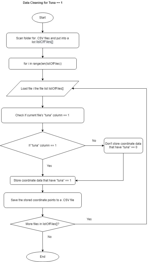
This cleaner is used right after predicting the data through SVM to check whether the data contains a column that has tuna == 1 or tuna == 0.

yesTunaCleaner.py

This cleaner works in a similar way by iterating through the predicted data folder, cleaning the data, and then saving the new cleaned data files in a new folder.

Functionalities

for i in range(len(listOfFiles)):
    cleanFile(defaultFolderDirectory+folderOfDataToClean +
              listOfFiles[i], cleanedFolderPath)
print("Successfully cleaned", len(listOfFiles), "files")

The function above takes the original folder that contains the files to clean and then a list of files that are in the folder and the output folder directory. This is the main function that we created in order to clean a single file and save it in the target file. Therefore to clean all the files in the folder, in the script we created a for loop to call this function according to all of the files that exists in our folder.

    for i in range(0, len(dataFrameLatLngSource["lat"])):

        if dataFrameLatLngSource["tuna"][i] == 1:
            # access first dataframe index (after header)
            listOfLat.append(dataFrameLatLngSource["lat"][i])
            listOfLng.append(dataFrameLatLngSource["lon"][i])

            listOfSST.append(dataFrameLatLngSource["sst"][i])  # new
            listOfChlorophyll.append(
                dataFrameLatLngSource["chlorophyll"][i])  # new
            listOfTuna.append(dataFrameLatLngSource["tuna"][i]) #new tuna

The snippet above shows how the data is checked if it contains the column "tuna" == 1. If it does, then the data that corresponds to that iteration is stored in the appropriate lists.

    dataCoba = {"lat": listOfLat,
                "lon": listOfLng,
                "sst": listOfSST,
                "chlorophyll": listOfChlorophyll,
                "tuna": listOfTuna}
    dataFrameCoba = pd.DataFrame(dataCoba)

The code above shows how all of the lists that contains the stored coordinate dadta is combined together into a single dataframe so that it can be saved to a CSV in the next step.

  try:
        dataFrameCoba.to_csv(
            str(".\\"+targetFolderForCleanedFiles+"\\"+sourceFile[-14:]), index=False)
        print("Data saved successfuly to", str(
            ".\\"+targetFolderForCleanedFiles+"\\"+sourceFile[-14:]))
    except Exception as e:
        print("Error: failed to save to csv :( \n", e)  # TODO: Fix this

THe snippet aboves shows how a dataframe is saved into a csv file according to the source file's original filename into the target folder.

Prediction and SVM

Support Vector Machine (SVM)

SVM is one of the methods used in machine learning. SVM use hyperplane to classify data and separate them into different classes. In this project we use SVM to classify whether that coordinate has tuna or not. In SVM there are kernel that is used when data not linearly separable so we project from 2D to 3D so we can separate them. In this project we use RBF kernel because each coordinate is being plot close to each other so we want to be able to separate which coordinate has tuna or not accurately.

Our SVM Model

Because we want to predict tuna location using sea surface temperature and chlorophyll concentration, our SVM model become like this :

  (tuna ~ sst + chlorophyll, data = train, kernel = "radial")

We want to predict tuna location based on sst and chlorophyll using data training with variable train and with radial kernel or RBF.

Normalize the Training Data

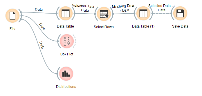
To make the prediction model, the first thing to do is preparing the training data. We can check the training data by looking at the distribution, we made the box plot and the distribution plot using Orange software.

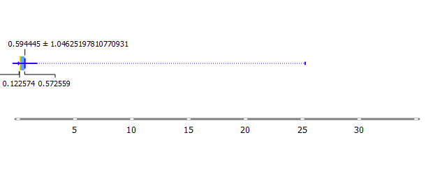
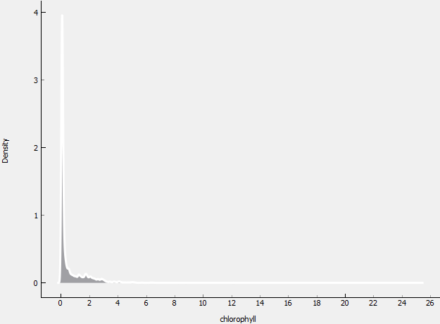
As we can see, the distribution of training data is not normal. This happened because there are several data with a very high value of chlorophyll (up to 3), while the average/mean is about 0.594445 and the median is 0.122574. To normalize the data, we select rows from data whose chlorophyll values are below 0.4 and then the selected data is stored in a new file in CSV format.

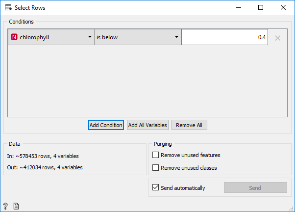
The selected data is 412034 rows from 578453 rows that will be used as training data. The Orange workflow can be seen below:

Making Predictions with Orange

From existing data, we can make a prediction model for predicting the existence of tuna. We can use Orange software to make the predictive model. First, we do a test and score to see the accuracy of the predictive model that we will make. As explained earlier, the method that we use to create a predictive model is SVM. Orange use Nu-SVC type for its SVM model. Model is trained with the following parameters:

Kernel: RBF
Cost: 1
Gamma: 0.03

Cost with value 1 and Gamma with value 0.03 is set by the same configuration as default svm function in R which has cost parameter with default value of 1 and Gamma with default value 1/(data dimension).

We do train by random sampling with a training set size 80% from training data that we have.

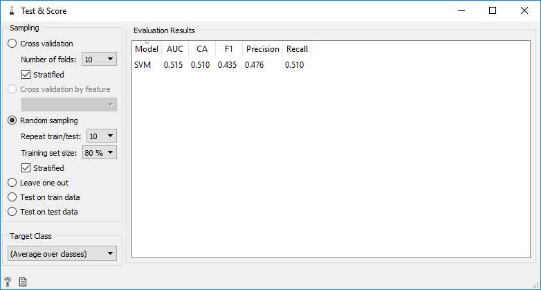
The resulting classification accuracy is 0.51, which means that the resulting predictive model still makes a lot of mistakes in making predictions. After seeing the accuracy, we make a predictive model. We do random sampling from training data (example 80% of training data) then train SVM model. After that, input the data that will be predicted into the model. In Orange, we have to enter data that will be predicted one by one. For example, we entered data on 01-01-2016 as data to be predicted. The model will generate predictions for each row of data. Then the results can be saved into a new file in CSV format. The Orange workflow can be seen below:

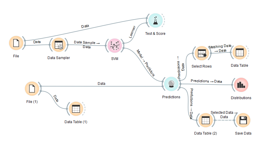
From the experiments we did on Orange, we saw that the predictive model we made in Orange has a small accuracy score. Besides that in Orange, we can't do file iteration, while our data consists of many files.

Making Predictions with Python

Because of Orange's limitations, we switch from it and use Python instead. We write a python script to create the predictive model and also making predictions. Python libraries that we use are as follows:

os: for operating system functionality. We use it to read a list of files from a directory.
pandas: for data manipulation and analysis.
sklearn.model_selection.train_test_split: for sampling data.
sklearn.svm.SVC: for making prediction model using SVM method.
sklearn.metrics.accuracy_score: for testing the model and checking the accuracy.
numpy: for scientific computing.
pickle: for saving and loading the resulting prediction model.

The method that we use to create a predictive model is SVM. We use sklearn package to make a predictive model. Sklearn use C-SVC type for its SVM model. Model are trained with the following parameters:

Kernel: RBF
Cost: 1
Gamma: 0.03

We make 3 types of prediction models, model that trained using 60% of training data, 70% of training data, and 80% of training data. We also calculate and compare the accuracy of each model by using the rest of the training data as testing data. The accuracy results are as follows:

	Accuracy
60% Training Data	70% Training Data	80% Training Data
0.7538558617593165	0.7527728114811788	0.7529093402259517

The python script to make prediction model can be seen below:

from sklearn import svm
from sklearn.model_selection.train_test_split
from sklearn.metrics.accuracy_score

# split the training data, for example: 40% of training data for training and 60% of training data for testing
x_train, x_test, y_train, y_test = train_test_split(x_training, y_training, test_size = 0.40)

# create a new SVM model
svmModel = svm.SVC(kernel='rbf', C=1 ,gamma=0.03, verbose=1)

# train the SVM model
svmModel.fit(x_train, y_train)

# test the accuracy of the model
y_svm = svmModel.predict(x_test)
print("Accuracy score: ", accuracy_score(y_test, y_svm))

The model saved into SAV file format and then we can load it to make a prediction:

import pickle

# save the model as a finalized_model_60.sav for example
filename = 'finalized_model_60.sav'
pickle.dump(svmModel, open(filename, 'wb'))

# load the model
svmModel = pickle.load(open("finalized_model_60.sav", 'rb'))

We predict the existence of tuna from 1 January 2012 until 31 December 2016 by using the data that has been cleaned before. The existence of tuna is indicated by tuna value=1, and if there is no tuna then tuna value=0. The results of the predictions are saved into the CSV file and placed into a folder. The predicted data now can be visualized by python dash.

Dash Dashboard with Bootstrap

Dash is a framework that allows us to build beautiful, web-based analytics applications. Through dash and its dash-core-components, we are able to create interactive elements that build up our interactive dashboard. In addition to that, this project also implements the bootstrap framework through the dash-bootstrap-components additional module in order to assist with the front-end development of the layout and design of the dashboard.

Setting up the Dash app

In order to show the data that we have produced into a map, we used MapBox's map API which needs an access token that can be requested on this link. Then with the API token, replace the variable below to your API token.

mapbox_access_token = "INSERT ACCESS TOKEN HERE"

The first part of the dash app consists of scanning the chosen folder that contains all of the coordinate information and then placing it into a list "listOfFiles[]. By default the folder loaded is the actual data (not trained) because that is the default first data that is shown on the dashboard.

listOfFiles = []
# by default the "." value will make it the current working directory of the py file
defaultFolderDirectory = "."
currentChosenPredictionModel = "\\actual\\"
try:
    # change me
    for folderName, subFolders, fileNames in os.walk(defaultFolderDirectory+currentChosenPredictionModel):
        # print("The filenames in "+folderName+" are: "+str(fileNames))
        for files in fileNames:
            listOfFiles.append(files)
    print("\nSuccessfuly loaded List of Files:",
          len(listOfFiles), "files total")

Next is the essential part where we create the variables that contains the components that will be placed into the dashboard. These components are made of the dash-core-components and dash-bootstrap-components that are provided in the modules we imported previously. In the snippet below the dash-core-components can be seen by the prefix "dcc." and the dash-bootstrap-components can be seen with the prefix "dbc.". Dash also supports html elements such as html.P, html.H1, html.Div,html.Hr, and more and so certain HTML elements are used to create the overall layout of the dashboard.

logoTuna = dbc.Navbar(
    dbc.Container(
        [html.A(
            ...
            dbc.NavbarToggler(id="navbar-toggler2"),
            dbc.Collapse(
                dbc.Nav(
                    ...
                        ...
                    ], c...
                ),
topCards = dbc.Container(
    [dbc.Row(
            [..    dbc.Col(dbc.Card(...
                    dbc.CardBody(...
body = dbc.Container(
    [dbc.Row(
            [...
                dbc.Col(...
                    [       ..[               
tableBottom = dbc.Container(
    [dbc.Row(
            [dbc.Col([
                    html.Div([
                        html.Hr(),
                        html.H3("Coordinates Table"),
                        ....

After creating the variables that will house the components for the dashboard, we need to setup dash to recognize the python script as a dash app. Since Dash supports the use of CSS, and since we are also using the bootstrap framework, we used an external CSS file in order to help make the application more user friendly. Also we can change the title that appears on the browser to a custom title which we changed accordingly.

app = dash.Dash(__name__, external_stylesheets=[dbc.themes.COSMO])
app.title = "Tuna Fish Forecaster"

Now that dash recognizes that the python script is a dash app, we can then input all of the variables that contained the components created previously into the dash app's layout. At the end, we also added an additional html.Div with extra information to demonstrate that it is also possible to add components wihtout creating a variable.

app.layout = html.Div([  
    logoTuna,
    topCards,
    body,
    tableBottom,

    # -----
    html.Div([
        html.P('Developed by Deananda Irwansyah, Christopher Yefta, & James Adhitthana',
               style={'display': 'inline'})
    ], className="twelve columns", style={'fontSize': 18, 'padding-top': 20, 'textAlign': 'center'}
    ),
])

Now that the layout and view is all set up, we must create the callbacks which basically handles all of the main functionality of each of the interactable components in the app and sets where the output is for each callback. For every callback, it must first start with an "@app.callback"() function that contains the parameters for at least one dash.dependencies.Output component which are components such as labels/tables/maps/graphs/any other component that needs to receive input data. The function also must recieve at least one dash.dependencies.Input component such as a slider/dropdown/any other component that can be manipulated by the user.

After every "@app.callback()" function, it must then be directly followed underneath by a function that recieves the parameters of the inputs that we have set up in the dash.dependencies.Input values. Then this function can be filled with the intended functionalities. By the end of this function, it must return the variables according to the dash.dependencies.Output we hav previously set up according to the order given.

#---Callback Slider to Data Table---#
@app.callback(
    # set the output as the checkbox's options
    [dash.dependencies.Output("tableFish", "data"),
     dash.dependencies.Output("labelChosenDate", "children"),
     dash.dependencies.Output("numberOfTunaLocationsInSelection", "children"),
     # dash.dependencies.Output("datePicker", "date"),
     ],
    # set the iniput as the radiobutton's values
    [dash.dependencies.Input("dateSlider", "value"),
     dash.dependencies.Input("dropdownPredictionModel", "value"), ]
    #     [dash.dependencies.Input("tableFish", "data"),
    #  dash.dependencies.Input("labelChosenDate", "children"), ])
)
def changeDate(selector, valueDropdown):
    ...
    return data, labelBaru, labelNumberOfTunaLocationsInSelection  # ,dateBaru


#---------Callback Dropdown to Slider---------#
@app.callback(
    # set the output as the checkbox's options
    [  # dash.dependencies.Output("dateSlider", "marks"),
        dash.dependencies.Output("dateSlider", "max"),
        dash.dependencies.Output("dateSlider", "min")],
    # set the iniput as the radiobutton's values
    [dash.dependencies.Input("dropdownYear", "value"),
     # dash.dependencies.Input("datePicker", "date")
     ]
)
def changeYear(selector):  # , datePickerDate):
    ...
      return maxDate, minDate
      
#---------Callback Mapbox---------#      
@app.callback(
    dash.dependencies.Output("map-graph", "figure"),  # output to map graph
    [dash.dependencies.Input("tableFish", "data"),
     dash.dependencies.Input("labelChosenDate", "children"), ])  # input from dropdown list
def update_graph(data, labelChosenDate):      
      ...
      return {"data": trace1, "layout": layout1}
      
      
#---Callback dropdown prediction model---#
@app.callback(
    # set the output as the checkbox's options
    dash.dependencies.Output("labelChosenPredictionModel", "children"),
    # set the iniput as the radiobutton's values
    [dash.dependencies.Input("dropdownPredictionModel", "value"), ]
)
def changeLabelChosenPredictionModel(selector):  # , datePickerDate):
    labelBaru = selector  # change label
    return labelBaru

Now that all of the essential functionality of the app is created, this snippet essentially runs the dash app when the python script is executed.

if __name__ == "__main__":
    app.run_server(debug=True)

Built With

Python - Python Programming Language
Dash - Dash
Dash Bootstrap Components - Bootstrap components on Dash
Cosmo - Bootstrap theme
Plotly - Plotly graph
Mapbox - Mapbox Map API
Orange - Orange Data Mining Toolbox
Scikit-learn - Scikit-learn
Pandas - Pandas
Numpy - Numpy

Authors

Christopher Yefta - ChrisYef
Deananda Irwansyah - hikariyoru
James Adhitthana - jamesadhitthana

License

This project is licensed under the MIT License - see the LICENSE file for details

Acknowledgments

Fishing vessel data in csv format by Global Fishing Watch
sst data in netCDF format by NOAA
chlorophyll concentration data in netCDF format by OceanWatch
Table of decimal degrees Decimal degrees

jamesadhitthana / TunaForecaster

Tuna Prediction

Introduction

Getting Started

Prerequisites

Running the application

Explanation

Data Cleansing

tunaDataCleanerSSTChlorophyll.py

#--How to use--#

Functionalities

Data Cleansing Part 2

yesTunaCleaner.py

Functionalities

Prediction and SVM

Support Vector Machine (SVM)

Our SVM Model

Normalize the Training Data

Making Predictions with Orange

Making Predictions with Python

Dash Dashboard with Bootstrap

Setting up the Dash app

Built With

Authors

License

Acknowledgments

References

About

Languages

References

- All India Survey on Higher Education. Guidelines for Filling Geographical Referencing Details. PDF. India: Government of India.
- Scikit-learn: Machine Learning in Python, Pedregosa et al., JMLR 12, pp. 2825-2830, 2011.
- Demsar J, Curk T, Erjavec A, Gorup C, Hocevar T, Milutinovic M, Mozina M, Polajnar M, Toplak M, Staric A, Stajdohar M, Umek L, Zagar L, Zbontar J, Zitnik M, Zupan B (2013) Orange: Data Mining Toolbox in Python, Journal of Machine Learning Research 14(Aug): 2349−2353.
- Stéfan van der Walt, S. Chris Colbert and Gaël Varoquaux. The NumPy Array: A Structure for Efficient Numerical Computation, Computing in Science & Engineering, 13, 22-30 (2011), DOI:10.1109/MCSE.2011.37
- Chih-Chung Chang and Chih-Jen Lin, LIBSVM : a library for support vector machines. ACM Transactions on Intelligent Systems and Technology, 2:27:1--27:27, 2011. Software available at http://www.csie.ntu.edu.tw/~cjlin/libsvm
- Wes McKinney. Data Structures for Statistical Computing in Python, Proceedings of the 9th Python in Science Conference, 51-56 (2010)