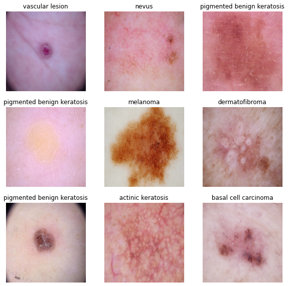
Problem statement: To build a CNN based model which can accurately detect melanoma. Melanoma is a type of cancer that can be deadly if not detected early. It accounts for 75% of skin cancer deaths. A solution which can evaluate images and alert the dermatologists about the presence of melanoma has the potential to reduce a lot of manual effort needed in diagnosis.
import pathlib
import tensorflow as tf
import matplotlib.pyplot as plt
import numpy
import pandas as pd
import os
import PIL
from tensorflow import keras
from tensorflow.keras import layers
from tensorflow.keras.models import Sequential
## If you are using the data by mounting the google drive, use the following :
## from google.colab import drive
## drive.mount('/content/gdrive')
##Ref:https://towardsdatascience.com/downloading-datasets-into-google-drive-via-google-colab-bcb1b30b0166This assignment uses a dataset of about 2357 images of skin cancer types. The dataset contains 9 sub-directories in each train and test subdirectories. The 9 sub-directories contains the images of 9 skin cancer types respectively.
# Defining the path for train and test images
## Todo: Update the paths of the train and test dataset
data_dir_train = pathlib.Path(r"Skin cancer ISIC The International Skin Imaging Collaboration\Train")
data_dir_test = pathlib.Path(r"Skin cancer ISIC The International Skin Imaging Collaboration\Test")
image_count_train = len(list(data_dir_train.glob('*/*.jpg')))
print(image_count_train)
image_count_test = len(list(data_dir_test.glob('*/*.jpg')))
print(image_count_test)2239
118
Let's load these images off disk using the helpful image_dataset_from_directory utility.
Defining some parameters for the loader:
batch_size = 32
img_height = 180
img_width = 180
Use 80% of the images for training, and 20% for validation.
## Write your train dataset here
## Note use seed=123 while creating your dataset using tf.keras.preprocessing.image_dataset_from_directory
## Note, make sure your resize your images to the size img_height*img_width, while writting the dataset
train_ds = tf.keras.preprocessing.image_dataset_from_directory(
  data_dir_train,
  validation_split=0.2,
  subset="training",
  seed=123,
  image_size=(img_height, img_width),
  batch_size=batch_size)
Found 2239 files belonging to 9 classes.
Using 1792 files for training.
## Write your validation dataset here
## Note use seed=123 while creating your dataset using tf.keras.preprocessing.image_dataset_from_directory
## Note, make sure your resize your images to the size img_height*img_width, while writting the dataset
val_ds = tf.keras.preprocessing.image_dataset_from_directory(
  data_dir_train,
  validation_split=0.2,
  subset="validation",
  seed=123,
  image_size=(img_height, img_width),
  batch_size=batch_size)
Found 2239 files belonging to 9 classes.
Using 447 files for validation.
# List out all the classes of skin cancer and store them in a list.
# You can find the class names in the class_names attribute on these datasets.
# These correspond to the directory names in alphabetical order.
class_names = train_ds.class_names
print(class_names)
['actinic keratosis', 'basal cell carcinoma', 'dermatofibroma', 'melanoma', 'nevus', 'pigmented benign keratosis', 'seborrheic keratosis', 'squamous cell carcinoma', 'vascular lesion']
import matplotlib.pyplot as plt

plt.figure(figsize=(10, 10))
for images, labels in train_ds.take(1):
  for i in range(9):
    ax = plt.subplot(3, 3, i + 1)
    plt.imshow(images[i].numpy().astype("uint8"))
    plt.title(class_names[labels[i]])
    plt.axis("off")
The image_batch is a tensor of the shape (32, 180, 180, 3). This is a batch of 32 images of shape 180x180x3 (the last dimension refers to color channels RGB). The label_batch is a tensor of the shape (32,), these are corresponding labels to the 32 images.
Dataset.cache() keeps the images in memory after they're loaded off disk during the first epoch.
Dataset.prefetch() overlaps data preprocessing and model execution while training.
AUTOTUNE = tf.data.experimental.AUTOTUNE
train_ds = train_ds.cache().shuffle(1000).prefetch(buffer_size=AUTOTUNE)
val_ds = val_ds.cache().prefetch(buffer_size=AUTOTUNE)
Creating a CNN model, which can accurately detect 9 classes present in the dataset. Using layers.experimental.preprocessing.Rescaling to normalize pixel values between (0,1). The RGB channel values are in the [0, 255] range. This is not ideal for a neural network. Here, it is good to standardize values to be in the [0, 1]
num_classes = 9

model = Sequential([
  layers.experimental.preprocessing.Rescaling(1./255, input_shape=(img_height, img_width, 3)),
  layers.Conv2D(16, 3, padding='same', activation='relu'),
  layers.MaxPooling2D(),
  layers.Conv2D(32, 3, padding='same', activation='relu'),
  layers.MaxPooling2D(),
  layers.Conv2D(64, 3, padding='same', activation='relu'),
  layers.MaxPooling2D(),
  layers.Flatten(),
  layers.Dense(128, activation='relu'),
  layers.Dense(num_classes,activation='softmax')
])Choose an appropirate optimiser and loss function for model training
### Todo, choose an appropirate optimiser and loss function
model.compile(optimizer='adam',
              loss=tf.keras.losses.SparseCategoricalCrossentropy(),
              metrics=['accuracy'])
# View the summary of all layers
model.summary()Model: "sequential_22"
_________________________________________________________________
Layer (type) Output Shape Param #
=================================================================
rescaling_16 (Rescaling) (None, 180, 180, 3) 0
_________________________________________________________________
conv2d_60 (Conv2D) (None, 180, 180, 16) 448
_________________________________________________________________
max_pooling2d_60 (MaxPooling (None, 90, 90, 16) 0
_________________________________________________________________
conv2d_61 (Conv2D) (None, 90, 90, 32) 4640
_________________________________________________________________
max_pooling2d_61 (MaxPooling (None, 45, 45, 32) 0
_________________________________________________________________
conv2d_62 (Conv2D) (None, 45, 45, 64) 18496
_________________________________________________________________
max_pooling2d_62 (MaxPooling (None, 22, 22, 64) 0
_________________________________________________________________
flatten_16 (Flatten) (None, 30976) 0
_________________________________________________________________
dense_32 (Dense) (None, 128) 3965056
_________________________________________________________________
dense_33 (Dense) (None, 9) 1161
=================================================================
Total params: 3,989,801
Trainable params: 3,989,801
Non-trainable params: 0
_________________________________________________________________
epochs = 20
history = model.fit(
  train_ds,
  validation_data=val_ds,
  epochs=epochs
)
Epoch 1/20
56/56 [==============================] - 28s 402ms/step - loss: 1.9937 - accuracy: 0.2651 - val_loss: 1.7181 - val_accuracy: 0.4407
Epoch 2/20
56/56 [==============================] - 22s 389ms/step - loss: 1.6267 - accuracy: 0.4124 - val_loss: 1.5865 - val_accuracy: 0.4295
Epoch 3/20
56/56 [==============================] - 21s 378ms/step - loss: 1.4485 - accuracy: 0.4860 - val_loss: 1.4204 - val_accuracy: 0.4922
Epoch 4/20
56/56 [==============================] - 22s 391ms/step - loss: 1.3651 - accuracy: 0.5184 - val_loss: 1.3913 - val_accuracy: 0.5257
Epoch 5/20
56/56 [==============================] - 21s 377ms/step - loss: 1.2641 - accuracy: 0.5396 - val_loss: 1.3957 - val_accuracy: 0.5436
Epoch 6/20
56/56 [==============================] - 21s 378ms/step - loss: 1.1883 - accuracy: 0.5792 - val_loss: 1.5191 - val_accuracy: 0.5123
Epoch 7/20
56/56 [==============================] - 21s 378ms/step - loss: 1.1650 - accuracy: 0.5809 - val_loss: 1.4289 - val_accuracy: 0.5526
Epoch 8/20
56/56 [==============================] - 21s 376ms/step - loss: 1.0380 - accuracy: 0.6423 - val_loss: 1.4168 - val_accuracy: 0.4966
Epoch 9/20
56/56 [==============================] - 21s 375ms/step - loss: 1.0041 - accuracy: 0.6406 - val_loss: 1.4042 - val_accuracy: 0.5213
Epoch 10/20
56/56 [==============================] - 21s 379ms/step - loss: 0.9185 - accuracy: 0.6724 - val_loss: 1.3424 - val_accuracy: 0.5705
Epoch 11/20
56/56 [==============================] - 21s 376ms/step - loss: 0.8762 - accuracy: 0.6735 - val_loss: 1.6004 - val_accuracy: 0.5414
Epoch 12/20
56/56 [==============================] - 21s 375ms/step - loss: 0.7715 - accuracy: 0.7148 - val_loss: 1.5463 - val_accuracy: 0.5593
Epoch 13/20
56/56 [==============================] - 21s 378ms/step - loss: 0.6433 - accuracy: 0.7656 - val_loss: 1.6616 - val_accuracy: 0.5682
Epoch 14/20
56/56 [==============================] - 21s 377ms/step - loss: 0.5490 - accuracy: 0.8075 - val_loss: 1.5744 - val_accuracy: 0.5145
Epoch 15/20
56/56 [==============================] - 21s 376ms/step - loss: 0.5284 - accuracy: 0.8092 - val_loss: 1.6828 - val_accuracy: 0.5481
Epoch 16/20
56/56 [==============================] - 21s 382ms/step - loss: 0.5035 - accuracy: 0.8214 - val_loss: 1.9489 - val_accuracy: 0.5123
Epoch 17/20
56/56 [==============================] - 21s 380ms/step - loss: 0.4565 - accuracy: 0.8320 - val_loss: 2.1713 - val_accuracy: 0.5682
Epoch 18/20
56/56 [==============================] - 21s 376ms/step - loss: 0.4863 - accuracy: 0.8281 - val_loss: 1.9792 - val_accuracy: 0.5593
Epoch 19/20
56/56 [==============================] - 21s 382ms/step - loss: 0.3406 - accuracy: 0.8750 - val_loss: 2.0060 - val_accuracy: 0.5145
Epoch 20/20
56/56 [==============================] - 21s 378ms/step - loss: 0.2891 - accuracy: 0.8901 - val_loss: 2.4874 - val_accuracy: 0.5391
acc = history.history['accuracy']
val_acc = history.history['val_accuracy']

loss = history.history['loss']
val_loss = history.history['val_loss']

epochs_range = range(epochs)

plt.figure(figsize=(8, 8))
plt.subplot(1, 2, 1)
plt.plot(epochs_range, acc, label='Training Accuracy')
plt.plot(epochs_range, val_acc, label='Validation Accuracy')
plt.legend(loc='lower right')
plt.title('Training and Validation Accuracy')

plt.subplot(1, 2, 2)
plt.plot(epochs_range, loss, label='Training Loss')
plt.plot(epochs_range, val_loss, label='Validation Loss')
plt.legend(loc='upper right')
plt.title('Training and Validation Loss')
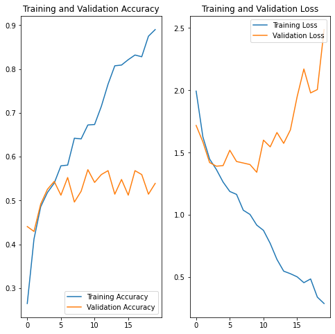
plt.show()As we can see that the training accuracy is increasing after every epoch and goes up to 91% but the validation accuracy gets stuck arround 53% after a few epoch. To deal with this problem we will.
-
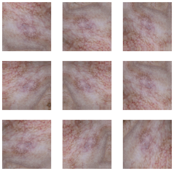
- Random Rotation
- Random Flipping
- Random Zooming
# Todo, after you have analysed the model fit history for presence of underfit or overfit, choose an appropriate data augumentation strategy.
data_augmentation = keras.Sequential(
  [
    layers.experimental.preprocessing.RandomRotation(1),
    layers.experimental.preprocessing.RandomZoom(0.1),
    layers.experimental.preprocessing.RandomFlip("horizontal",input_shape=(img_height, img_width,3))
  ]
)
# Todo, visualize how your augmentation strategy works for one instance of training image.
plt.figure(figsize=(10, 10))
for images, _ in train_ds.take(1):
for i in range(9):
augmented_images = data_augmentation(images)
ax = plt.subplot(3, 3, i + 1)
plt.imshow(augmented_images[0].numpy().astype("uint8"))
plt.axis("off")## You can use Dropout layer if there is an evidence of overfitting in your findings
model = Sequential([
data_augmentation,
layers.experimental.preprocessing.Rescaling(1./255),
layers.Conv2D(16, 3, padding='same', activation='relu'),
layers.MaxPooling2D(),
layers.Dropout(0.2),
layers.Conv2D(32, 3, padding='same', activation='relu'),
layers.MaxPooling2D(),
layers.Dropout(0.2),
layers.Conv2D(64, 3, padding='same', activation='relu'),
layers.MaxPooling2D(),
layers.Dropout(0.2),
layers.Conv2D(128, 3, padding='same', activation='relu'),
layers.MaxPooling2D(),
layers.Dropout(0.2),
layers.Flatten(),
layers.Dense(256, activation='relu'),
layers.Dropout(0.3),
layers.Dense(num_classes, activation='softmax')
])model.compile(optimizer='adam',
loss=tf.keras.losses.SparseCategoricalCrossentropy(),
metrics=['accuracy'])## Your code goes here, note: train your model for 20 epochs
epochs = 20
history = model.fit(
train_ds,
validation_data=val_ds,
epochs=epochs
)Epoch 1/20
56/56 [==============================] - 34s 573ms/step - loss: 2.0455 - accuracy: 0.2310 - val_loss: 1.9159 - val_accuracy: 0.2908
Epoch 2/20
56/56 [==============================] - 32s 571ms/step - loss: 1.8082 - accuracy: 0.3404 - val_loss: 1.8727 - val_accuracy: 0.3289
Epoch 3/20
56/56 [==============================] - 34s 600ms/step - loss: 1.7190 - accuracy: 0.3817 - val_loss: 1.7670 - val_accuracy: 0.3758
Epoch 4/20
56/56 [==============================] - 34s 614ms/step - loss: 1.6651 - accuracy: 0.3906 - val_loss: 1.5959 - val_accuracy: 0.4519
Epoch 5/20
56/56 [==============================] - 33s 598ms/step - loss: 1.6098 - accuracy: 0.4146 - val_loss: 1.5974 - val_accuracy: 0.4609
Epoch 6/20
56/56 [==============================] - 32s 571ms/step - loss: 1.5971 - accuracy: 0.4247 - val_loss: 1.6374 - val_accuracy: 0.4206
Epoch 7/20
56/56 [==============================] - 32s 564ms/step - loss: 1.4732 - accuracy: 0.4805 - val_loss: 1.5597 - val_accuracy: 0.4452
Epoch 8/20
56/56 [==============================] - 32s 574ms/step - loss: 1.4514 - accuracy: 0.5056 - val_loss: 1.5357 - val_accuracy: 0.4452
Epoch 9/20
56/56 [==============================] - 34s 612ms/step - loss: 1.4277 - accuracy: 0.5022 - val_loss: 1.5431 - val_accuracy: 0.4497
Epoch 10/20
56/56 [==============================] - 34s 610ms/step - loss: 1.4240 - accuracy: 0.5039 - val_loss: 1.4518 - val_accuracy: 0.4922
Epoch 11/20
56/56 [==============================] - 32s 571ms/step - loss: 1.3738 - accuracy: 0.5173 - val_loss: 1.7345 - val_accuracy: 0.3714
Epoch 12/20
56/56 [==============================] - 32s 566ms/step - loss: 1.3715 - accuracy: 0.5195 - val_loss: 1.4371 - val_accuracy: 0.4899
Epoch 13/20
56/56 [==============================] - 32s 564ms/step - loss: 1.3516 - accuracy: 0.5257 - val_loss: 1.5993 - val_accuracy: 0.4094
Epoch 14/20
56/56 [==============================] - 33s 598ms/step - loss: 1.3291 - accuracy: 0.5290 - val_loss: 1.4127 - val_accuracy: 0.4966
Epoch 15/20
56/56 [==============================] - 34s 612ms/step - loss: 1.3785 - accuracy: 0.5112 - val_loss: 1.3684 - val_accuracy: 0.4944
Epoch 16/20
56/56 [==============================] - 33s 593ms/step - loss: 1.3209 - accuracy: 0.5268 - val_loss: 1.6102 - val_accuracy: 0.4228
Epoch 17/20
56/56 [==============================] - 32s 570ms/step - loss: 1.3187 - accuracy: 0.5385 - val_loss: 1.3932 - val_accuracy: 0.4922
Epoch 18/20
56/56 [==============================] - 32s 564ms/step - loss: 1.2920 - accuracy: 0.5312 - val_loss: 1.3865 - val_accuracy: 0.5123
Epoch 19/20
56/56 [==============================] - 32s 572ms/step - loss: 1.2764 - accuracy: 0.5413 - val_loss: 1.5668 - val_accuracy: 0.4966
Epoch 20/20
56/56 [==============================] - 34s 615ms/step - loss: 1.2920 - accuracy: 0.5329 - val_loss: 1.6381 - val_accuracy: 0.3937
acc = history.history['accuracy']
val_acc = history.history['val_accuracy']

loss = history.history['loss']
val_loss = history.history['val_loss']

epochs_range = range(epochs)

plt.figure(figsize=(8, 8))
plt.subplot(1, 2, 1)
plt.plot(epochs_range, acc, label='Training Accuracy')
plt.plot(epochs_range, val_acc, label='Validation Accuracy')
plt.legend(loc='lower right')
plt.title('Training and Validation Accuracy')

plt.subplot(1, 2, 2)
plt.plot(epochs_range, loss, label='Training Loss')
plt.plot(epochs_range, val_loss, label='Validation Loss')
plt.legend(loc='upper right')
plt.title('Training and Validation Loss')
plt.show()
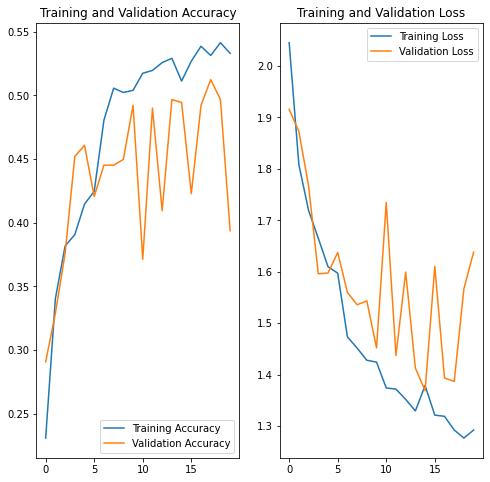
The gap between training and testing accuracy has decreased but the overall accuracy of the model did not improve. We will check for class imballance in the dataset.
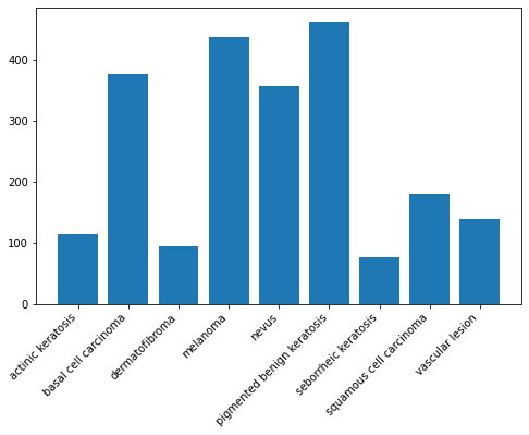
Context: Many times real life datasets can have class imbalance, one class can have proportionately higher number of samples compared to the others. Class imbalance can have a detrimental effect on the final model quality. Hence as a sanity check it becomes important to check what is the distribution of classes in the data.
plt.figure(figsize=(8, 5))
plt.xticks(rotation=45, ha="right")
plt.bar(x=class_names,height=[len(list(data_dir_train.glob(c+'/*.jpg'))) for c in class_names])
<BarContainer object of 9 artists>
Context: You can use a python package known as Augmentor (https://augmentor.readthedocs.io/en/master/) to add more samples across all classes so that none of the classes have very few samples.
!pip install AugmentorRequirement already satisfied: Augmentor in c:\users\prakhar\anaconda3\lib\site-packages (0.2.8)
Requirement already satisfied: Pillow>=5.2.0 in c:\users\prakhar\anaconda3\lib\site-packages (from Augmentor) (8.0.1)
Requirement already satisfied: numpy>=1.11.0 in c:\users\prakhar\anaconda3\lib\site-packages (from Augmentor) (1.20.3)
Requirement already satisfied: future>=0.16.0 in c:\users\prakhar\anaconda3\lib\site-packages (from Augmentor) (0.18.2)
Requirement already satisfied: tqdm>=4.9.0 in c:\users\prakhar\anaconda3\lib\site-packages (from Augmentor) (4.50.2)
To use Augmentor, the following general procedure is followed:
- Instantiate a
Pipelineobject pointing to a directory containing your initial image data set. - Define a number of operations to perform on this data set using your
Pipelineobject. - Execute these operations by calling the
Pipeline’ssample()method.
path_to_training_dataset= r"Skin cancer ISIC The International Skin Imaging Collaboration\Train\\"
import Augmentor
for i in class_names:
    p = Augmentor.Pipeline(path_to_training_dataset + i)
    p.rotate(probability=0.7, max_left_rotation=10, max_right_rotation=10)
    p.sample(500) ## We are adding 500 samples per class to make sure that none of the classes are sparse.
Executing Pipeline: 0%| | 0/500 [00:00<?, ? Samples/s]
Initialised with 114 image(s) found.
Output directory set to Skin cancer ISIC The International Skin Imaging Collaboration\Train\\actinic keratosis\output.
Processing <PIL.Image.Image image mode=RGB size=600x450 at 0x20FDA7F7D30>: 100%|█| 500/500 [00:04<00:00, 103.92 Samples
Executing Pipeline: 0%| | 0/500 [00:00<?, ? Samples/s]
Initialised with 376 image(s) found.
Output directory set to Skin cancer ISIC The International Skin Imaging Collaboration\Train\\basal cell carcinoma\output.
Processing <PIL.Image.Image image mode=RGB size=600x450 at 0x20FDA906940>: 100%|█| 500/500 [00:05<00:00, 99.86 Samples/
Processing <PIL.Image.Image image mode=RGB size=600x450 at 0x20FDA9AE4C0>: 0%| | 0/500 [00:00<?, ? Samples/s]
Initialised with 95 image(s) found.
Output directory set to Skin cancer ISIC The International Skin Imaging Collaboration\Train\\dermatofibroma\output.
Processing <PIL.JpegImagePlugin.JpegImageFile image mode=RGB size=600x450 at 0x20FA2297FD0>: 100%|█| 500/500 [00:05<00:
Executing Pipeline: 0%| | 0/500 [00:00<?, ? Samples/s]
Initialised with 438 image(s) found.
Output directory set to Skin cancer ISIC The International Skin Imaging Collaboration\Train\\melanoma\output.
Processing <PIL.JpegImagePlugin.JpegImageFile image mode=RGB size=3072x2304 at 0x20F8958E520>: 100%|█| 500/500 [00:25<0
Executing Pipeline: 0%| | 0/500 [00:00<?, ? Samples/s]
Initialised with 357 image(s) found.
Output directory set to Skin cancer ISIC The International Skin Imaging Collaboration\Train\\nevus\output.
Processing <PIL.Image.Image image mode=RGB size=3072x2304 at 0x20F9C174AC0>: 100%|█| 500/500 [00:21<00:00, 22.80 Sample
Processing <PIL.Image.Image image mode=RGB size=600x450 at 0x20F86E5CD90>: 3%| | 16/500 [00:00<00:26, 18.05 Samples/s
Initialised with 462 image(s) found.
Output directory set to Skin cancer ISIC The International Skin Imaging Collaboration\Train\\pigmented benign keratosis\output.
Processing <PIL.Image.Image image mode=RGB size=600x450 at 0x20FA3EC0310>: 100%|█| 500/500 [00:04<00:00, 110.59 Samples
Executing Pipeline: 0%| | 0/500 [00:00<?, ? Samples/s]
Initialised with 77 image(s) found.
Output directory set to Skin cancer ISIC The International Skin Imaging Collaboration\Train\\seborrheic keratosis\output.
Processing <PIL.Image.Image image mode=RGB size=1024x768 at 0x20FD926C430>: 100%|█| 500/500 [00:10<00:00, 48.41 Samples
Processing <PIL.JpegImagePlugin.JpegImageFile image mode=RGB size=600x450 at 0x20F9F556490>: 2%| | 8/500 [00:00<00:26
Initialised with 181 image(s) found.
Output directory set to Skin cancer ISIC The International Skin Imaging Collaboration\Train\\squamous cell carcinoma\output.
Processing <PIL.Image.Image image mode=RGB size=600x450 at 0x20F9862EDC0>: 100%|█| 500/500 [00:04<00:00, 114.77 Samples
Processing <PIL.Image.Image image mode=RGB size=600x450 at 0x20F9F25B880>: 0%| | 1/500 [00:00<01:25, 5.83 Samples/s]
Initialised with 139 image(s) found.
Output directory set to Skin cancer ISIC The International Skin Imaging Collaboration\Train\\vascular lesion\output.
Processing <PIL.Image.Image image mode=RGB size=600x450 at 0x20FA0E09B80>: 100%|█| 500/500 [00:04<00:00, 109.22 Samples
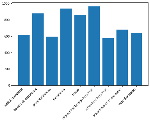
Augmentor has stored the augmented images in the output sub-directory of each of the sub-directories of skin cancer types.. Lets take a look at total count of augmented images.
image_count_train = len(list(data_dir_train.glob('*/output/*.jpg')))
print(image_count_train)
4500
# path_list = [x for x in data_dir_train.glob(os.path.join('*','output', '*.jpg'))]
# path_list_new = path_list
# lesion_list_new = [os.path.basename(os.path.dirname(os.path.dirname(y))) for y in data_dir_train.glob(os.path.join('*','output', '*.jpg'))]
# lesion_list_new# dataframe_dict_new = dict(zip(path_list_new, lesion_list_new))# df2 = pd.DataFrame(list(dataframe_dict_new.items()),columns = ['Path','Label'])
# new_df = original_df.append(df2)# new_df['Label'].value_counts()plt.figure(figsize=(8, 5))
plt.xticks(rotation=45, ha="right")
plt.bar(x=class_names,height=[len(list(data_dir_train.glob(c+'/*.jpg'))) + len(list(data_dir_train.glob(c+'/output/*.jpg'))) for c in class_names])<BarContainer object of 9 artists>
So, now we have added 500 images to all the classes to maintain some class balance. We can add more images as we want to improve training process.
batch_size = 32
img_height = 180
img_width = 180# data_dir_train="path to directory with training data + data created using augmentor"
train_ds = tf.keras.preprocessing.image_dataset_from_directory(
data_dir_train,
seed=123,
validation_split = 0.2,
subset = "training",
image_size=(img_height, img_width),
batch_size=batch_size)Found 6739 files belonging to 9 classes.
Using 5392 files for training.
val_ds = tf.keras.preprocessing.image_dataset_from_directory(
  data_dir_train,
  seed=123,
  validation_split = 0.2,
  subset = 'validation',
  image_size=(img_height, img_width),
  batch_size=batch_size)
Found 6739 files belonging to 9 classes.
Using 1347 files for validation.
model = Sequential([
  layers.experimental.preprocessing.Rescaling(1./255),
  layers.Conv2D(16, 3, padding='same', activation='relu'),
  layers.MaxPooling2D(),
  layers.Dropout(0.2),
  layers.Conv2D(32, 3, padding='same', activation='relu'),
  layers.MaxPooling2D(),
  layers.Dropout(0.2),
  layers.Conv2D(64, 3, padding='same', activation='relu'),
  layers.MaxPooling2D(),
  layers.Dropout(0.2),
  layers.Conv2D(128, 3, padding='same', activation='relu'),
  layers.MaxPooling2D(),
  layers.Dropout(0.2),
  layers.Flatten(),
  layers.Dense(256, activation='relu'),
  layers.Dropout(0.3),
  layers.Dense(num_classes, activation='softmax')
])model.compile(optimizer='adam',
loss=tf.keras.losses.SparseCategoricalCrossentropy(),
metrics=['accuracy'])epochs = 30
history = model.fit(
train_ds,
validation_data=val_ds,
epochs=epochs
)Epoch 1/30
169/169 [==============================] - 106s 617ms/step - loss: 2.0144 - accuracy: 0.2120 - val_loss: 1.9336 - val_accuracy: 0.3170
Epoch 2/30
169/169 [==============================] - 98s 575ms/step - loss: 1.7341 - accuracy: 0.3388 - val_loss: 1.7268 - val_accuracy: 0.3682
Epoch 3/30
169/169 [==============================] - 99s 585ms/step - loss: 1.5227 - accuracy: 0.4201 - val_loss: 1.5581 - val_accuracy: 0.4016
Epoch 4/30
169/169 [==============================] - 97s 571ms/step - loss: 1.4630 - accuracy: 0.4425 - val_loss: 1.4459 - val_accuracy: 0.4402
Epoch 5/30
169/169 [==============================] - 100s 591ms/step - loss: 1.3049 - accuracy: 0.4959 - val_loss: 1.4026 - val_accuracy: 0.4454
Epoch 6/30
169/169 [==============================] - 96s 565ms/step - loss: 1.2468 - accuracy: 0.5245 - val_loss: 1.2513 - val_accuracy: 0.5108
Epoch 7/30
169/169 [==============================] - 100s 587ms/step - loss: 1.1454 - accuracy: 0.5645 - val_loss: 1.4298 - val_accuracy: 0.4388
Epoch 8/30
169/169 [==============================] - 97s 571ms/step - loss: 1.0739 - accuracy: 0.5886 - val_loss: 1.0624 - val_accuracy: 0.6028
Epoch 9/30
169/169 [==============================] - 99s 584ms/step - loss: 0.9409 - accuracy: 0.6384 - val_loss: 0.9205 - val_accuracy: 0.6555
Epoch 10/30
169/169 [==============================] - 98s 577ms/step - loss: 0.8511 - accuracy: 0.6749 - val_loss: 0.8903 - val_accuracy: 0.6689
Epoch 11/30
169/169 [==============================] - 98s 580ms/step - loss: 0.7801 - accuracy: 0.7055 - val_loss: 0.8626 - val_accuracy: 0.6882
Epoch 12/30
169/169 [==============================] - 99s 581ms/step - loss: 0.6924 - accuracy: 0.7381 - val_loss: 0.7751 - val_accuracy: 0.7275
Epoch 13/30
169/169 [==============================] - 98s 575ms/step - loss: 0.6406 - accuracy: 0.7596 - val_loss: 0.6992 - val_accuracy: 0.7446
Epoch 14/30
169/169 [==============================] - 100s 589ms/step - loss: 0.5667 - accuracy: 0.7821 - val_loss: 0.6897 - val_accuracy: 0.7476
Epoch 15/30
169/169 [==============================] - 97s 571ms/step - loss: 0.5657 - accuracy: 0.7862 - val_loss: 0.8502 - val_accuracy: 0.7045
Epoch 16/30
169/169 [==============================] - 100s 592ms/step - loss: 0.5159 - accuracy: 0.8025 - val_loss: 0.6574 - val_accuracy: 0.7610
Epoch 17/30
169/169 [==============================] - 97s 569ms/step - loss: 0.4809 - accuracy: 0.8171 - val_loss: 0.6509 - val_accuracy: 0.7632
Epoch 18/30
169/169 [==============================] - 100s 589ms/step - loss: 0.4202 - accuracy: 0.8370 - val_loss: 0.6502 - val_accuracy: 0.7713
Epoch 19/30
169/169 [==============================] - 97s 574ms/step - loss: 0.4262 - accuracy: 0.8383 - val_loss: 0.6341 - val_accuracy: 0.7854
Epoch 20/30
169/169 [==============================] - 99s 584ms/step - loss: 0.4262 - accuracy: 0.8390 - val_loss: 0.5984 - val_accuracy: 0.8018
Epoch 21/30
169/169 [==============================] - 99s 585ms/step - loss: 0.3598 - accuracy: 0.8566 - val_loss: 0.5747 - val_accuracy: 0.8107
Epoch 22/30
169/169 [==============================] - 98s 578ms/step - loss: 0.3526 - accuracy: 0.8615 - val_loss: 0.5802 - val_accuracy: 0.8270
Epoch 23/30
169/169 [==============================] - 99s 582ms/step - loss: 0.3349 - accuracy: 0.8728 - val_loss: 0.6128 - val_accuracy: 0.7921
Epoch 24/30
169/169 [==============================] - 97s 572ms/step - loss: 0.3490 - accuracy: 0.8646 - val_loss: 0.6528 - val_accuracy: 0.8055
Epoch 25/30
169/169 [==============================] - 99s 586ms/step - loss: 0.3237 - accuracy: 0.8717 - val_loss: 0.6191 - val_accuracy: 0.8159
Epoch 26/30
169/169 [==============================] - 96s 567ms/step - loss: 0.2778 - accuracy: 0.8956 - val_loss: 0.6256 - val_accuracy: 0.8300
Epoch 27/30
169/169 [==============================] - 100s 592ms/step - loss: 0.3155 - accuracy: 0.8802 - val_loss: 0.5663 - val_accuracy: 0.8367
Epoch 28/30
169/169 [==============================] - 97s 569ms/step - loss: 0.3578 - accuracy: 0.8633 - val_loss: 0.5655 - val_accuracy: 0.8404
Epoch 29/30
169/169 [==============================] - 99s 586ms/step - loss: 0.2816 - accuracy: 0.8895 - val_loss: 0.6446 - val_accuracy: 0.8151
Epoch 30/30
169/169 [==============================] - 97s 573ms/step - loss: 0.2691 - accuracy: 0.8993 - val_loss: 0.5226 - val_accuracy: 0.8411
acc = history.history['accuracy']
val_acc = history.history['val_accuracy']

loss = history.history['loss']
val_loss = history.history['val_loss']

epochs_range = range(epochs)

plt.figure(figsize=(8, 8))
plt.subplot(1, 2, 1)
plt.plot(epochs_range, acc, label='Training Accuracy')
plt.plot(epochs_range, val_acc, label='Validation Accuracy')
plt.legend(loc='lower right')
plt.title('Training and Validation Accuracy')

plt.subplot(1, 2, 2)
plt.plot(epochs_range, loss, label='Training Loss')
plt.plot(epochs_range, val_loss, label='Validation Loss')
plt.legend(loc='upper right')
plt.title('Training and Validation Loss')
plt.show()
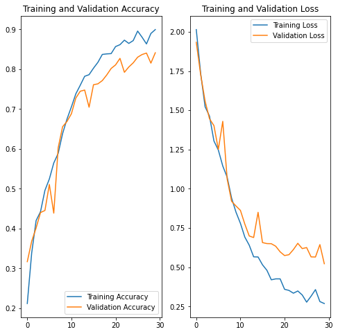
Todo: Analyze your results here. Did you get rid of underfitting/overfitting? Did class rebalance help?
After performing augumentation, both training as well as the validation accuracies improved significantly. and we have a model with decent accuracy.
