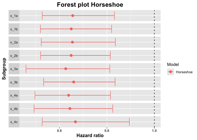
Subgroup analyses are routinely performed in clinical trial analyses. From a methodological perspective, two key issues of subgroup analyses are multiplicity (even if only predefined subgroups are investigated) and the low sample sizes of subgroups which lead to highly variable estimates, see e.g. Yusuf et al (1991). This package implements subgroup estimates based on Bayesian shrinkage priors, see Carvalho et al (2019). In addition, estimates based on penalized likelihood inference are available, based on Simon et al (2011). The corresponding shrinkage based forest plots address the aforementioned issues and can complement standard forest plots in practical clinical trial analyses.
Please note that on Windows, you will need to install
Rtools, because you
will need to have a working C++ toolchain to compile the Stan models.
You can install the current release version of bonsaiforest from CRAN
with:
install.packages("bonsaiforest")You can install the development version of bonsaiforest from
GitHub with:
# install.packages("remotes")
remotes::install_github("insightsengineering/bonsaiforest")See the introductory vignette or get started by trying out the example:
library(bonsaiforest)
str(example_data)
#> 'data.frame':    1000 obs. of  14 variables:
#>  $ id    : int  1 2 3 4 5 6 7 8 9 10 ...
#>  $ arm   : Factor w/ 2 levels "0","1": 1 1 1 1 2 2 2 2 2 1 ...
#>  $ x_1   : Factor w/ 2 levels "a","b": 2 2 1 1 2 1 1 2 2 1 ...
#>  $ x_2   : Factor w/ 2 levels "a","b": 1 2 1 1 1 2 2 1 2 2 ...
#>  $ x_3   : Factor w/ 2 levels "a","b": 2 1 2 1 2 2 2 1 2 2 ...
#>  $ x_4   : Factor w/ 3 levels "a","b","c": 2 1 3 3 3 3 3 1 3 3 ...
#>  $ x_5   : Factor w/ 4 levels "a","b","c","d": 4 4 1 1 4 1 3 4 4 3 ...
#>  $ x_6   : Factor w/ 2 levels "a","b": 2 1 2 2 2 1 2 2 2 2 ...
#>  $ x_7   : Factor w/ 2 levels "a","b": 2 1 2 2 2 1 1 2 2 2 ...
#>  $ x_8   : Factor w/ 3 levels "a","b","c": 3 2 1 3 3 3 1 1 2 3 ...
#>  $ x_9   : Factor w/ 2 levels "a","b": 2 1 2 2 2 1 1 2 2 2 ...
#>  $ x_10  : Factor w/ 3 levels "a","b","c": 3 3 3 3 3 1 2 2 2 3 ...
#>  $ tt_pfs: num  0.9795 3.4762 1.7947 0.0197 2.2168 ...
#>  $ ev_pfs: num  1 0 1 1 0 0 0 0 0 0 ...
horseshoe_model <- horseshoe(
resp = "tt_pfs", trt = "arm",
subgr = c("x_1", "x_2", "x_3", "x_4"),
covars = c(
"x_1", "x_2", "x_3", "x_4", "x_5",
"x_6", "x_7", "x_8", "x_9", "x_10"
),
data = example_data, resptype = "survival",
status = "ev_pfs", chains = 2, seed = 0,
control = list(adapt_delta = 0.95)
)
#> Compiling Stan program...
#> Start sampling
#>
#> SAMPLING FOR MODEL 'anon_model' NOW (CHAIN 1).
#> Chain 1:
#> Chain 1: Gradient evaluation took 0.00022 seconds
#> Chain 1: 1000 transitions using 10 leapfrog steps per transition would take 2.2 seconds.
#> Chain 1: Adjust your expectations accordingly!
#> Chain 1:
#> Chain 1:
#> Chain 1: Iteration: 1 / 2000 [ 0%] (Warmup)
#> Chain 1: Iteration: 200 / 2000 [ 10%] (Warmup)
#> Chain 1: Iteration: 400 / 2000 [ 20%] (Warmup)
#> Chain 1: Iteration: 600 / 2000 [ 30%] (Warmup)
#> Chain 1: Iteration: 800 / 2000 [ 40%] (Warmup)
#> Chain 1: Iteration: 1000 / 2000 [ 50%] (Warmup)
#> Chain 1: Iteration: 1001 / 2000 [ 50%] (Sampling)
#> Chain 1: Iteration: 1200 / 2000 [ 60%] (Sampling)
#> Chain 1: Iteration: 1400 / 2000 [ 70%] (Sampling)
#> Chain 1: Iteration: 1600 / 2000 [ 80%] (Sampling)
#> Chain 1: Iteration: 1800 / 2000 [ 90%] (Sampling)
#> Chain 1: Iteration: 2000 / 2000 [100%] (Sampling)
#> Chain 1:
#> Chain 1: Elapsed Time: 9.899 seconds (Warm-up)
#> Chain 1: 7.865 seconds (Sampling)
#> Chain 1: 17.764 seconds (Total)
#> Chain 1:
#>
#> SAMPLING FOR MODEL 'anon_model' NOW (CHAIN 2).
#> Chain 2:
#> Chain 2: Gradient evaluation took 0.000117 seconds
#> Chain 2: 1000 transitions using 10 leapfrog steps per transition would take 1.17 seconds.
#> Chain 2: Adjust your expectations accordingly!
#> Chain 2:
#> Chain 2:
#> Chain 2: Iteration: 1 / 2000 [ 0%] (Warmup)
#> Chain 2: Iteration: 200 / 2000 [ 10%] (Warmup)
#> Chain 2: Iteration: 400 / 2000 [ 20%] (Warmup)
#> Chain 2: Iteration: 600 / 2000 [ 30%] (Warmup)
#> Chain 2: Iteration: 800 / 2000 [ 40%] (Warmup)
#> Chain 2: Iteration: 1000 / 2000 [ 50%] (Warmup)
#> Chain 2: Iteration: 1001 / 2000 [ 50%] (Sampling)
#> Chain 2: Iteration: 1200 / 2000 [ 60%] (Sampling)
#> Chain 2: Iteration: 1400 / 2000 [ 70%] (Sampling)
#> Chain 2: Iteration: 1600 / 2000 [ 80%] (Sampling)
#> Chain 2: Iteration: 1800 / 2000 [ 90%] (Sampling)
#> Chain 2: Iteration: 2000 / 2000 [100%] (Sampling)
#> Chain 2:
#> Chain 2: Elapsed Time: 10.131 seconds (Warm-up)
#> Chain 2: 7.004 seconds (Sampling)
#> Chain 2: 17.135 seconds (Total)
#> Chain 2:
#> Warning: There were 1 divergent transitions after warmup. See
#> https://mc-stan.org/misc/warnings.html#divergent-transitions-after-warmup
#> to find out why this is a problem and how to eliminate them.
#> Warning: Examine the pairs() plot to diagnose sampling problemssummary_horseshoe <- summary(horseshoe_model, conf = 0.9)
summary_horseshoe
#> subgroup trt.estimate trt.low trt.high
#> 1 x_1a 0.6557710 0.5269372 0.8319575
#> 2 x_1b 0.6497113 0.5195755 0.8197317
#> 3 x_2a 0.6545330 0.5229767 0.8356877
#> 4 x_2b 0.6493245 0.5202362 0.8144661
#> 5 x_3a 0.6262720 0.4585270 0.8121477
#> 6 x_3b 0.6597057 0.5328791 0.8345641
#> 7 x_4a 0.6385074 0.4967184 0.8150692
#> 8 x_4b 0.6438776 0.4929574 0.8245606
#> 9 x_4c 0.6673139 0.5271375 0.8948151plot(summary_horseshoe)
