In this lab, you'll further practice the ideas behind CNN and adapting pretrained models as described in previous lessons. (As you may have guessed, our problem at hand is classifying Santa or Not Santa!). With that, let's have at it!
You will be able to:
- Use Keras to adapt a pretrained CNN
- Implement feature engineering and fine tuning on a pretrained model
import datetime

start = datetime.datetime.now()
import os, shutil
import time
import matplotlib.pyplot as plt
import scipy
import numpy as np
from PIL import Image
from scipy import ndimage
from keras.preprocessing.image import ImageDataGenerator, array_to_img
np.random.seed(123)/Users/matthew.mitchell/anaconda3/lib/python3.6/site-packages/h5py/__init__.py:36: FutureWarning: Conversion of the second argument of issubdtype from `float` to `np.floating` is deprecated. In future, it will be treated as `np.float64 == np.dtype(float).type`.
from ._conv import register_converters as _register_converters
Using TensorFlow backend.
train_folder = 'split/train'
test_folder = 'split/test'
val_folder = 'split/validation'
datagen = ImageDataGenerator(rescale=1./255)
batch_size = 10from keras.applications import VGG19
cnn_base = VGG19(weights='imagenet',
include_top=False,
input_shape=(64, 64, 3))cnn_base.summary()_________________________________________________________________
Layer (type) Output Shape Param #
=================================================================
input_1 (InputLayer) (None, 64, 64, 3) 0
_________________________________________________________________
block1_conv1 (Conv2D) (None, 64, 64, 64) 1792
_________________________________________________________________
block1_conv2 (Conv2D) (None, 64, 64, 64) 36928
_________________________________________________________________
block1_pool (MaxPooling2D) (None, 32, 32, 64) 0
_________________________________________________________________
block2_conv1 (Conv2D) (None, 32, 32, 128) 73856
_________________________________________________________________
block2_conv2 (Conv2D) (None, 32, 32, 128) 147584
_________________________________________________________________
block2_pool (MaxPooling2D) (None, 16, 16, 128) 0
_________________________________________________________________
block3_conv1 (Conv2D) (None, 16, 16, 256) 295168
_________________________________________________________________
block3_conv2 (Conv2D) (None, 16, 16, 256) 590080
_________________________________________________________________
block3_conv3 (Conv2D) (None, 16, 16, 256) 590080
_________________________________________________________________
block3_conv4 (Conv2D) (None, 16, 16, 256) 590080
_________________________________________________________________
block3_pool (MaxPooling2D) (None, 8, 8, 256) 0
_________________________________________________________________
block4_conv1 (Conv2D) (None, 8, 8, 512) 1180160
_________________________________________________________________
block4_conv2 (Conv2D) (None, 8, 8, 512) 2359808
_________________________________________________________________
block4_conv3 (Conv2D) (None, 8, 8, 512) 2359808
_________________________________________________________________
block4_conv4 (Conv2D) (None, 8, 8, 512) 2359808
_________________________________________________________________
block4_pool (MaxPooling2D) (None, 4, 4, 512) 0
_________________________________________________________________
block5_conv1 (Conv2D) (None, 4, 4, 512) 2359808
_________________________________________________________________
block5_conv2 (Conv2D) (None, 4, 4, 512) 2359808
_________________________________________________________________
block5_conv3 (Conv2D) (None, 4, 4, 512) 2359808
_________________________________________________________________
block5_conv4 (Conv2D) (None, 4, 4, 512) 2359808
_________________________________________________________________
block5_pool (MaxPooling2D) (None, 2, 2, 512) 0
=================================================================
Total params: 20,024,384
Trainable params: 20,024,384
Non-trainable params: 0
_________________________________________________________________
def extract_features(directory, sample_amount):
    features = np.zeros(shape=(sample_amount, 2, 2, 512))
    labels = np.zeros(shape=(sample_amount))
    generator = datagen.flow_from_directory(
        directory, target_size=(64, 64),
        batch_size = 10,
        class_mode='binary')
    i=0
    for inputs_batch, labels_batch in generator:
        features_batch = cnn_base.predict(inputs_batch)
        features[i * batch_size : (i + 1) * batch_size] = features_batch
        labels[i * batch_size : (i + 1) * batch_size] = labels_batch
        i = i + 1
        if i * batch_size >= sample_amount:
            break
    return features, labels
# you should be able to divide sample_amount by batch_size!!
train_features, train_labels = extract_features(train_folder, 540)
validation_features, validation_labels = extract_features(val_folder, 200)
test_features, test_labels = extract_features(test_folder, 180)
train_features = np.reshape(train_features, (540, 2 * 2 * 512))
validation_features = np.reshape(validation_features, (200, 2 * 2 * 512))
test_features = np.reshape(test_features, (180, 2 * 2 * 512))Found 542 images belonging to 2 classes.
Found 200 images belonging to 2 classes.
Found 180 images belonging to 2 classes.
from keras import models
from keras import layers
from keras import optimizers

model = models.Sequential()
model.add(layers.Dense(256, activation='relu', input_dim=2 * 2 * 512))
model.add(layers.Dense(1, activation='sigmoid'))

model.compile(optimizer=optimizers.RMSprop(lr=1e-4),
              loss='binary_crossentropy',
              metrics=['acc'])
history = model.fit(train_features, train_labels,
                    epochs=20,
                    batch_size=10,
                    validation_data=(validation_features, validation_labels))
Train on 540 samples, validate on 200 samples
Epoch 1/20
540/540 [==============================] - 0s 822us/step - loss: 0.4196 - acc: 0.8370 - val_loss: 0.2900 - val_acc: 0.9150
Epoch 2/20
540/540 [==============================] - 0s 430us/step - loss: 0.2363 - acc: 0.9167 - val_loss: 0.1999 - val_acc: 0.9300
Epoch 3/20
540/540 [==============================] - 0s 427us/step - loss: 0.1742 - acc: 0.9370 - val_loss: 0.1683 - val_acc: 0.9400
Epoch 4/20
540/540 [==============================] - 0s 431us/step - loss: 0.1371 - acc: 0.9593 - val_loss: 0.1583 - val_acc: 0.9400
Epoch 5/20
540/540 [==============================] - 0s 476us/step - loss: 0.1136 - acc: 0.9574 - val_loss: 0.1527 - val_acc: 0.9400
Epoch 6/20
540/540 [==============================] - 0s 434us/step - loss: 0.0964 - acc: 0.9704 - val_loss: 0.1444 - val_acc: 0.9450
Epoch 7/20
540/540 [==============================] - 0s 432us/step - loss: 0.0794 - acc: 0.9778 - val_loss: 0.1381 - val_acc: 0.9350
Epoch 8/20
540/540 [==============================] - 0s 430us/step - loss: 0.0674 - acc: 0.9852 - val_loss: 0.1368 - val_acc: 0.9400
Epoch 9/20
540/540 [==============================] - 0s 446us/step - loss: 0.0548 - acc: 0.9907 - val_loss: 0.1366 - val_acc: 0.9350
Epoch 10/20
540/540 [==============================] - 0s 435us/step - loss: 0.0511 - acc: 0.9889 - val_loss: 0.1353 - val_acc: 0.9350
Epoch 11/20
540/540 [==============================] - 0s 489us/step - loss: 0.0422 - acc: 0.9926 - val_loss: 0.1464 - val_acc: 0.9450
Epoch 12/20
540/540 [==============================] - 0s 441us/step - loss: 0.0361 - acc: 0.9944 - val_loss: 0.1347 - val_acc: 0.9450
Epoch 13/20
540/540 [==============================] - 0s 435us/step - loss: 0.0301 - acc: 0.9981 - val_loss: 0.1387 - val_acc: 0.9350
Epoch 14/20
540/540 [==============================] - 0s 430us/step - loss: 0.0262 - acc: 0.9944 - val_loss: 0.1414 - val_acc: 0.9300
Epoch 15/20
540/540 [==============================] - 0s 451us/step - loss: 0.0220 - acc: 1.0000 - val_loss: 0.1389 - val_acc: 0.9400
Epoch 16/20
540/540 [==============================] - 0s 427us/step - loss: 0.0176 - acc: 1.0000 - val_loss: 0.1420 - val_acc: 0.9450
Epoch 17/20
540/540 [==============================] - 0s 447us/step - loss: 0.0163 - acc: 1.0000 - val_loss: 0.1536 - val_acc: 0.9300
Epoch 18/20
540/540 [==============================] - 0s 425us/step - loss: 0.0119 - acc: 1.0000 - val_loss: 0.1475 - val_acc: 0.9350
Epoch 19/20
540/540 [==============================] - 0s 427us/step - loss: 0.0114 - acc: 1.0000 - val_loss: 0.1581 - val_acc: 0.9350
Epoch 20/20
540/540 [==============================] - 0s 427us/step - loss: 0.0089 - acc: 1.0000 - val_loss: 0.1699 - val_acc: 0.9350
results_test = model.evaluate(test_features, test_labels)
results_test
180/180 [==============================] - 0s 59us/step
[0.23546737531820933, 0.933333334657881]
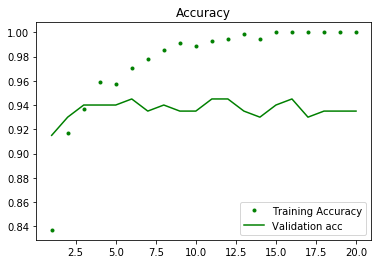
train_acc = history.history['acc']
val_acc = history.history['val_acc']
train_loss = history.history['loss']
val_loss = history.history['val_loss']
epch = range(1, len(train_acc) + 1)
plt.plot(epch, train_acc, 'g.', label='Training Accuracy')
plt.plot(epch, val_acc, 'g', label='Validation acc')
plt.title('Accuracy')
plt.legend()
plt.figure()
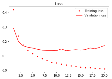
plt.plot(epch, train_loss, 'r.', label='Training loss')
plt.plot(epch, val_loss, 'r', label='Validation loss')
plt.title('Loss')
plt.legend()
plt.show()
Using VGG19 we were able to get test set performance up to almost 92%. Quite impressive!
end = datetime.datetime.now()
elapsed = end - start
print('Feature extraction method 1 took {} to execute.'.format(elapsed))
startp = datetime.datetime.now() #Set new start time for new process method
Feature extraction method 1 took 0:01:14.165131 to execute.
Here, we will investigate another method for performming feature extraction which will seque naturally into methods for fine tuning a pretrained network. This method of feature extraction is more costly then the previous methodology but has some added benefits in that it will allow us to also perform our usual data augmentation techniques.
Here's an overview of the process:
- Add the pretrained model as the first layer
- Add some dense layers for a classifier on top
- Freeze the convolutional base
- Train the model
The new part of this process which you are unfamiliar with is freezing layers. This means that all of the weights associated with that layer(s) will remain unchanged through the optimization process. Freezing the base is important as we wish to preserve the features encoded in this CNN base.
model = models.Sequential()
model.add(cnn_base)
model.add(layers.Flatten())
model.add(layers.Dense(132, activation='relu'))
model.add(layers.Dense(1, activation='sigmoid'))Now that we've designed the model architecture, we can go ahead and freeze the base. First, let's look at how to check whether layers are frozen or not:
#You can check whether a layer is trainable (or alter its setting) through the layer.trainable attribute:
for layer in model.layers:
    print(layer.name, layer.trainable)

#Similarly, we can check how many trainable weights are in the model:
print(len(model.trainable_weights))
vgg19 True
flatten_1 True
dense_3 True
dense_4 True
36
And now let's freeze our cnn base layer:
cnn_base.trainable = Falseand do a quick sanity check:
#You can check whether a layer is trainable (or alter its setting) through the layer.trainable attribute:
for layer in model.layers:
    print(layer.name, layer.trainable)

#Similarly, we can check how many trainable weights are in the model:
print(len(model.trainable_weights))
vgg19 False
flatten_1 True
dense_3 True
dense_4 True
4
From there, training the model happens as usual.
We define our training-validation-test sets (now with data augmentation; the advantage of this method of feature-extraction).
# get all the data in the directory split/train (542 images), and reshape them
train_datagen = ImageDataGenerator(
      rescale=1./255,
      rotation_range=40,
      width_shift_range=0.2,
      height_shift_range=0.2,
      shear_range=0.2,
      zoom_range=0.2,
      horizontal_flip=True,
      fill_mode='nearest')

train_generator = train_datagen.flow_from_directory(
        train_folder,
        target_size=(64, 64),
        batch_size= 20,
        class_mode= 'binary')

# get all the data in the directory split/validation (200 images), and reshape them
val_generator = ImageDataGenerator(rescale=1./255).flow_from_directory(
        val_folder,
        target_size=(64, 64),
        batch_size = 20,
        class_mode= 'binary')

# get all the data in the directory split/test (180 images), and reshape them
test_generator = ImageDataGenerator(rescale=1./255).flow_from_directory(
        test_folder,
        target_size=(64, 64),
        batch_size = 180,
        class_mode= 'binary')

test_images, test_labels = next(test_generator)
Found 542 images belonging to 2 classes.
Found 200 images belonging to 2 classes.
Found 180 images belonging to 2 classes.
Compile the model as usual:
model.compile(loss='binary_crossentropy',
              optimizer=optimizers.RMSprop(lr=2e-5),
              metrics=['acc'])
And fit the model:
history = model.fit_generator(
              train_generator,
              steps_per_epoch= 27,
              epochs = 10,
              validation_data = val_generator,
              validation_steps = 10)
Epoch 1/10
27/27 [==============================] - 36s 1s/step - loss: 0.7754 - acc: 0.5093 - val_loss: 0.6475 - val_acc: 0.5900
Epoch 2/10
27/27 [==============================] - 32s 1s/step - loss: 0.6349 - acc: 0.6168 - val_loss: 0.5764 - val_acc: 0.7550
Epoch 3/10
27/27 [==============================] - 33s 1s/step - loss: 0.5876 - acc: 0.7831 - val_loss: 0.5353 - val_acc: 0.7950
Epoch 4/10
27/27 [==============================] - 33s 1s/step - loss: 0.5558 - acc: 0.7991 - val_loss: 0.4962 - val_acc: 0.8850
Epoch 5/10
27/27 [==============================] - 34s 1s/step - loss: 0.5289 - acc: 0.8294 - val_loss: 0.4642 - val_acc: 0.8900
Epoch 6/10
27/27 [==============================] - 33s 1s/step - loss: 0.4927 - acc: 0.8467 - val_loss: 0.4414 - val_acc: 0.8700
Epoch 7/10
27/27 [==============================] - 33s 1s/step - loss: 0.4876 - acc: 0.8467 - val_loss: 0.4198 - val_acc: 0.8750
Epoch 8/10
27/27 [==============================] - 33s 1s/step - loss: 0.4591 - acc: 0.8523 - val_loss: 0.3878 - val_acc: 0.9150
Epoch 9/10
27/27 [==============================] - 33s 1s/step - loss: 0.4156 - acc: 0.8813 - val_loss: 0.3677 - val_acc: 0.9050
Epoch 10/10
27/27 [==============================] - 32s 1s/step - loss: 0.4012 - acc: 0.8869 - val_loss: 0.3430 - val_acc: 0.9300
train_acc = history.history['acc']
val_acc = history.history['val_acc']
train_loss = history.history['loss']
val_loss = history.history['val_loss']
epch = range(1, len(train_acc) + 1)
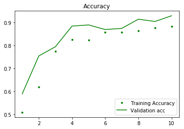
plt.plot(epch, train_acc, 'g.', label='Training Accuracy')
plt.plot(epch, val_acc, 'g', label='Validation acc')
plt.title('Accuracy')
plt.legend()
plt.figure()
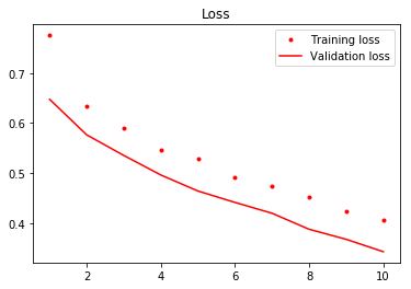
plt.plot(epch, train_loss, 'r.', label='Training loss')
plt.plot(epch, val_loss, 'r', label='Validation loss')
plt.title('Loss')
plt.legend()
plt.show()
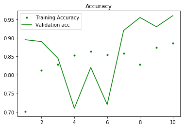
Comment: since both training and validation accuracy continue to fall in these graphs we would normally train for more epochs. To keep things running smoothly though, we won't do that here.
end = datetime.datetime.now()
elapsed = end - startp
print('Feature extraction method 2 took {} to execute.'.format(elapsed))
elapsed = end - start
print('Total running time of notebook thus far: {}'.format(elapsed))
startp = datetime.datetime.now() #Set new start time for new process method
Feature extraction method 2 took 0:18:45.504135 to execute.
Total running time of notebook thus far: 1:19:34.698920
Fine tuning starts with the same procedure that we have demonstrated for feature extraction. From there, we further fine-tune the weights of the most abstract layers of the convolutional base.
When fine-tuning these layers from the convolutional base, it is essential that you first freeze the entire convolutional base and train a classifier as we discussed with the feature engineering technique above. Without this, when gradient descent is initialized to optimize our loss function, we would be apt to loose any significant patterns learned by the original classifier that we are adapting to our current situation. As a result, we must first tune the fully-connected classifier that sits on top of the pretrained convolutional base. From there, our model should have a relatively strong accuracy and we can fine tune the weights of the last few layers of the convolutional base. Unfreezing initial layers of the convolutional base is not apt to produce substantial gains as these early layers typically learn simple representations such as colors and edges which are typically useful in all forms of image recognition, regardless of application.
With that, let's continue fine-tuning our model.
Warning: Fine tuning can be a resource intensive procedure.
Recall that we have our overall model:
model.summary()_________________________________________________________________
Layer (type) Output Shape Param #
=================================================================
vgg19 (Model) (None, 2, 2, 512) 20024384
_________________________________________________________________
flatten_1 (Flatten) (None, 2048) 0
_________________________________________________________________
dense_3 (Dense) (None, 132) 270468
_________________________________________________________________
dense_4 (Dense) (None, 1) 133
=================================================================
Total params: 270,601
Trainable params: 270,601
Non-trainable params: 0
_________________________________________________________________
/Users/matthew.mitchell/anaconda3/lib/python3.6/site-packages/keras/engine/training.py:490: UserWarning: Discrepancy between trainable weights and collected trainable weights, did you set `model.trainable` without calling `model.compile` after ?
'Discrepancy between trainable weights and collected trainable'
And we can also further investigate our borrowed convolutional base:
cnn_base.summary()_________________________________________________________________
Layer (type) Output Shape Param #
=================================================================
input_1 (InputLayer) (None, 64, 64, 3) 0
_________________________________________________________________
block1_conv1 (Conv2D) (None, 64, 64, 64) 1792
_________________________________________________________________
block1_conv2 (Conv2D) (None, 64, 64, 64) 36928
_________________________________________________________________
block1_pool (MaxPooling2D) (None, 32, 32, 64) 0
_________________________________________________________________
block2_conv1 (Conv2D) (None, 32, 32, 128) 73856
_________________________________________________________________
block2_conv2 (Conv2D) (None, 32, 32, 128) 147584
_________________________________________________________________
block2_pool (MaxPooling2D) (None, 16, 16, 128) 0
_________________________________________________________________
block3_conv1 (Conv2D) (None, 16, 16, 256) 295168
_________________________________________________________________
block3_conv2 (Conv2D) (None, 16, 16, 256) 590080
_________________________________________________________________
block3_conv3 (Conv2D) (None, 16, 16, 256) 590080
_________________________________________________________________
block3_conv4 (Conv2D) (None, 16, 16, 256) 590080
_________________________________________________________________
block3_pool (MaxPooling2D) (None, 8, 8, 256) 0
_________________________________________________________________
block4_conv1 (Conv2D) (None, 8, 8, 512) 1180160
_________________________________________________________________
block4_conv2 (Conv2D) (None, 8, 8, 512) 2359808
_________________________________________________________________
block4_conv3 (Conv2D) (None, 8, 8, 512) 2359808
_________________________________________________________________
block4_conv4 (Conv2D) (None, 8, 8, 512) 2359808
_________________________________________________________________
block4_pool (MaxPooling2D) (None, 4, 4, 512) 0
_________________________________________________________________
block5_conv1 (Conv2D) (None, 4, 4, 512) 2359808
_________________________________________________________________
block5_conv2 (Conv2D) (None, 4, 4, 512) 2359808
_________________________________________________________________
block5_conv3 (Conv2D) (None, 4, 4, 512) 2359808
_________________________________________________________________
block5_conv4 (Conv2D) (None, 4, 4, 512) 2359808
_________________________________________________________________
block5_pool (MaxPooling2D) (None, 2, 2, 512) 0
=================================================================
Total params: 20,024,384
Trainable params: 20,024,384
Non-trainable params: 0
_________________________________________________________________
Up till now, we have frozen the entire convolutional base. Again, it cannot be stressed enough how important this is before fine tuning the weights of the later layers of this base. Without training a classifier on the frozen base first, there will be too much noise in the model and initial epochs will overwrite any useful representations encoded in the pretrained model. That said, now that we have tuned a classifier to the frozen base, we can now unfreeze a few of the deeper layers from this base and further fine tune them to our problem scenario. In practice, this is apt to be particularly helpful where adapted models span new domain categories. For example, if the pretrained model is on cats and dogs and this is adapted to a problem specific to cats (a very relatively similar domain) there is apt to be little performance gain from fine tuning. On the other hand, if the problem domain is more substantially different, additional gains are more likely in adjusting these more abstract layers of the convolutional base. With that, let's take a look at how to unfreeze and fine tune these later layers.
Previously, we saw how to freeze a layer. Similarly, we will now unfreeze our base:
cnn_base.trainable = TrueThen, we can refreeze all of them up to a specific layer. Here we're unfreezing the final block of layers. (You will see diminishing returns if you continue to unfreeze additional layers.)
cnn_base.trainable = True
set_trainable = False
for layer in cnn_base.layers:
    if layer.name == 'block5_conv1':
        set_trainable = True
    if set_trainable:
        layer.trainable = True
    else:
        layer.trainable = False
Finally, we must recompile our model before performing fitting.
model.compile(loss='binary_crossentropy',
                      optimizer=optimizers.RMSprop(lr=1e-4),
                      metrics=['accuracy'])
Afterwards, we can then fit the model as usual.
history = model.fit_generator(
              train_generator,
              steps_per_epoch= 27,
              epochs = 10,
              validation_data = val_generator,
              validation_steps = 10)
Epoch 1/10
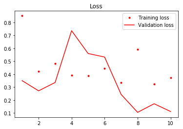
27/27 [==============================] - 43s 2s/step - loss: 0.8492 - acc: 0.6947 - val_loss: 0.3502 - val_acc: 0.8950
Epoch 2/10
27/27 [==============================] - 41s 2s/step - loss: 0.4234 - acc: 0.8130 - val_loss: 0.2716 - val_acc: 0.8900
Epoch 3/10
27/27 [==============================] - 40s 1s/step - loss: 0.4683 - acc: 0.8331 - val_loss: 0.3359 - val_acc: 0.8450
Epoch 4/10
27/27 [==============================] - 40s 1s/step - loss: 0.3880 - acc: 0.8572 - val_loss: 0.7360 - val_acc: 0.7100
Epoch 5/10
27/27 [==============================] - 40s 1s/step - loss: 0.3808 - acc: 0.8684 - val_loss: 0.5596 - val_acc: 0.8200
Epoch 6/10
27/27 [==============================] - 40s 1s/step - loss: 0.4314 - acc: 0.8591 - val_loss: 0.5324 - val_acc: 0.7200
Epoch 7/10
27/27 [==============================] - 39s 1s/step - loss: 0.3363 - acc: 0.8628 - val_loss: 0.2439 - val_acc: 0.9200
Epoch 8/10
27/27 [==============================] - 40s 1s/step - loss: 0.5722 - acc: 0.8331 - val_loss: 0.1054 - val_acc: 0.9550
Epoch 9/10
27/27 [==============================] - 40s 1s/step - loss: 0.3296 - acc: 0.8616 - val_loss: 0.1719 - val_acc: 0.9300
Epoch 10/10
27/27 [==============================] - 40s 1s/step - loss: 0.3616 - acc: 0.8888 - val_loss: 0.1117 - val_acc: 0.9600
train_acc = history.history['acc']
val_acc = history.history['val_acc']
train_loss = history.history['loss']
val_loss = history.history['val_loss']
epch = range(1, len(train_acc) + 1)
plt.plot(epch, train_acc, 'g.', label='Training Accuracy')
plt.plot(epch, val_acc, 'g', label='Validation acc')
plt.title('Accuracy')
plt.legend()
plt.figure()
plt.plot(epch, train_loss, 'r.', label='Training loss')
plt.plot(epch, val_loss, 'r', label='Validation loss')
plt.title('Loss')
plt.legend()
plt.show()As usual, let's conclude with a final evaluation on the test set.
# test_generator = test_datagen.flow_from_directory(
#         test_dir,
#         target_size=(150, 150),
#         batch_size=20,
#         class_mode='binary')
test_loss, test_acc = model.evaluate_generator(test_generator, steps=50)
print('test acc:', test_acc)
test acc: 0.9055555462837219
The model with fine-tuning seems to have similar results, but was much more costly to compute in terms of time.
In this lesson, you learned how to adapt a pretrained model to your own application. This can be a useful technique when data is limited (less then tens or hundreds of thousands of examples). To do this, you build a new classifier on top of the original convolutional base. Then, if the category or class of images is substantially different, fine tuning the most abstract layers of the convolutional base may further bolster performance. From here, it's time to fully synthesize all the image recognition techniques you have learned to date and practice with a real world example from a Kaggle competition.
