plumstan is an R package that computes age-depth models for sediment cores based on measured 210Pb activities using a Bayesian statistical framework.
This framework is developed and implemented in the R package plum by Aquino-López et al (2018). In contrast to plum, plumstan relies on the programming language Stan (Carpenter et al. 2017) in order to perform the Bayesian calculations. This has several advantages:
- MCMC sampling is efficient via
Stan's Hamiltonian Monte Carlo algorithm (Stan Development Team 2019). - The model can be modified and integrated into complex models more easily.
- The fitted model can be handled using the functions of the rstan package (Stan Development Team 2019)
Install plumstan with R:
remotes::install_github("henningte/plumstan")Load plumstan in R:
library("plumstan")Load the sample data (derived from the publication of Aquino-López et al (2018)) and inspect the first rows.
head(plumstan::ps_sample_data)
#>    type supported depth_lower depth_upper mass_density activity activity_sd age
#> 1 pb210     FALSE           1           0        0.045   371.73       11.90  NA
#> 2 pb210     FALSE           2           1        0.047   456.39       15.08  NA
#> 3 pb210     FALSE           3           2        0.051   454.24       17.11  NA
#> 4 pb210     FALSE           4           3        0.049   449.64       14.43  NA
#> 5 pb210     FALSE           5           4        0.049   479.04       16.44  NA
#> 6 pb210     FALSE           6           5        0.051   490.97       16.75  NA
#>   age_sd
#> 1     NA
#> 2     NA
#> 3     NA
#> 4     NA
#> 5     NA
#> 6     NA
For plumstan to use the data, it needs to be converted to an object of class ps_input.
d <- plumstan::ps_input(ps_sample_data)
class(d)
#> [1] "ps_input"   "data.frame"
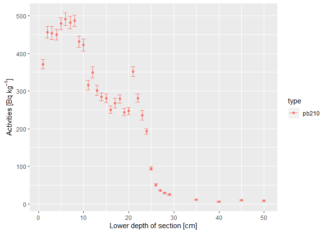
plumstan supports the visual identification of layers for which the background 210Pb activity is reached:
plot(d)For the last 4 sections, the background 210Pb activity level seems to be reached (Aquino-López et al. 2018). Therefore, the 210Pb activities of the last 4 sections can be used to estimate the supported 210Pb activity. Therefore, in d, column d$supported indicates that the deepest four layers should be used to estimate the supported 210Pb activity:
d$supported
#>  [1]  TRUE  TRUE  TRUE  TRUE FALSE FALSE FALSE FALSE FALSE FALSE FALSE FALSE
#> [13] FALSE FALSE FALSE FALSE FALSE FALSE FALSE FALSE FALSE FALSE FALSE FALSE
#> [25] FALSE FALSE FALSE FALSE FALSE FALSE FALSE FALSE FALSE
These data can be fed into the ps_get_model function. The function constructs a set of "artificial" depth layers wih fixed depth increments for the age-depth model and a Stan model. A thickness of the artificial sections of 1 cm is chosen.
d_model <- plumstan::ps_get_model(data_input = d, thickness = 1)ps_get_model constructs a ps_model object that contains the data and the compiled Stan model from which rstan's MCMC algorithm can sample.
plumstan_fit passes the data to rstan::stan in order to fit the Stan model contained in d_model. Thus, all options available for rstan::stan are also available for plumstan_fit.
d_fit <-
  plumstan::ps_fit_model(
    d_model,
    chains = 1,
    iter = 1500,
    warmup = 500,
    seed = 123)
#>
#> SAMPLING FOR MODEL 'plumstan_model' NOW (CHAIN 1).
#> Chain 1: Rejecting initial value:
#> Chain 1:   Log probability evaluates to log(0), i.e. negative infinity.
#> Chain 1:   Stan can't start sampling from this initial value.
#> Chain 1:
#> Chain 1: Gradient evaluation took 0 seconds
#> Chain 1: 1000 transitions using 10 leapfrog steps per transition would take 0 seconds.
#> Chain 1: Adjust your expectations accordingly!
#> Chain 1:
#> Chain 1:
#> Chain 1: Iteration:    1 / 1500 [  0%]  (Warmup)
#> Chain 1: Iteration:  150 / 1500 [ 10%]  (Warmup)
#> Chain 1: Iteration:  300 / 1500 [ 20%]  (Warmup)
#> Chain 1: Iteration:  450 / 1500 [ 30%]  (Warmup)
#> Chain 1: Iteration:  501 / 1500 [ 33%]  (Sampling)
#> Chain 1: Iteration:  650 / 1500 [ 43%]  (Sampling)
#> Chain 1: Iteration:  800 / 1500 [ 53%]  (Sampling)
#> Chain 1: Iteration:  950 / 1500 [ 63%]  (Sampling)
#> Chain 1: Iteration: 1100 / 1500 [ 73%]  (Sampling)
#> Chain 1: Iteration: 1250 / 1500 [ 83%]  (Sampling)
#> Chain 1: Iteration: 1400 / 1500 [ 93%]  (Sampling)
#> Chain 1: Iteration: 1500 / 1500 [100%]  (Sampling)
#> Chain 1:
#> Chain 1:  Elapsed Time: 2.518 seconds (Warm-up)
#> Chain 1:                1.388 seconds (Sampling)
#> Chain 1:                3.906 seconds (Total)
#> Chain 1:
d_fit is an object of class stanfit. Thus, all functions of the R packages rstan and bayesplot may be used in order to investigate and validate the fitted model.
The sediment age posterior predictive distributions (i.e. the MCMC samples after warmup) for each depth of the input sediment profile can be extracted as data.frame by passing d_model and d_fit to the function ps_extract_samples.
d_extracted_fit <-
  plumstan::ps_extract_samples(
    x = d_fit,
    ps_model = d_model)
d_extracted_fit is a data.frame containing the sampled parameter values (e.g. the estimated age values and Pb210 activites) for both the measured depth layers (d_extracted_fit$depth_profile == "measured") and the "artificial" depth profile (d_extracted_fit$depth_profile == "artificial"):
head(d_extracted_fit)
#>   iter data_type depth_profile depth_lower depth_upper      age
#> 1    1     pb210      measured          29          28 195.2209
#> 2    2     pb210      measured          29          28 204.5243
#> 3    3     pb210      measured          29          28 225.0797
#> 4    4     pb210      measured          29          28 194.0709
#> 5    5     pb210      measured          29          28 203.0467
#> 6    6     pb210      measured          29          28 191.2571
#>   depth_accumulation_rate depth_accumulation_rate_alpha pb210_tot
#> 1                      NA                            NA  14.20569
#> 2                      NA                            NA  13.25301
#> 3                      NA                            NA  13.91363
#> 4                      NA                            NA  15.45908
#> 5                      NA                            NA  16.10459
#> 6                      NA                            NA  14.54460
#>   pb210_supported     omega
#> 1      0.03834938 0.3076514
#> 2      0.03495767 0.3321187
#> 3      0.03514617 0.3319858
#> 4      0.03960609 0.3177757
#> 5      0.03571352 0.3012072
#> 6      0.03428386 0.3115710
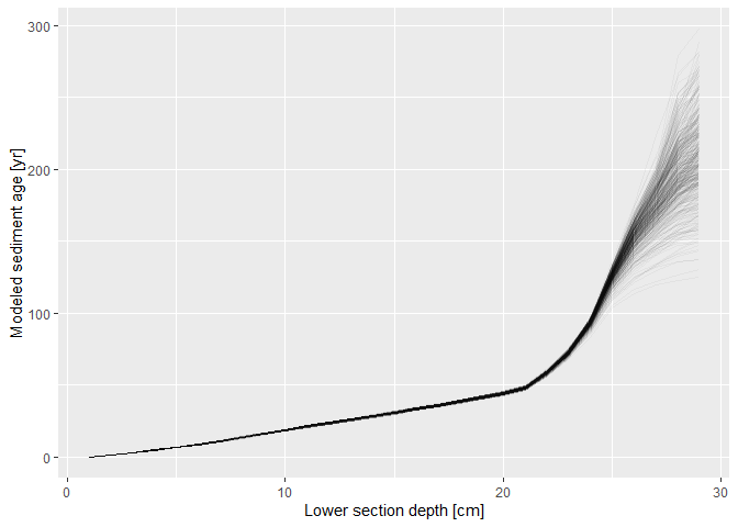
With d_extracted_fit, it is easy to plot the modeled age-depth profile, e.g. using functions of ggplot2: Here, I plotted the estimated sediment ages versus lower section depths according to the first 500 draws of the MCMC algorithm.
# load ggplot2
library(ggplot2)

# plot
ggplot(data = d_extracted_fit[d_extracted_fit$iter <= 500 & d_extracted_fit$depth_profile == "measured",],
       mapping = aes(x = depth_lower,
                     y = age,
                     group = iter)) +
  geom_path(alpha = 0.04) +
  labs(x = "Lower section depth [cm]",
       y = "Modeled sediment age [yr]")
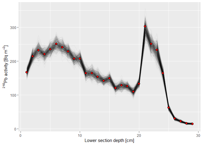
Similarly, the fitted total 210Pb activities can be visualised (red dots represent the measured 210Pb activities):
# plot
ggplot() +
  geom_path(data = d_extracted_fit[d_extracted_fit$iter <= 500 & d_extracted_fit$depth_profile == "measured",],
       mapping = aes(x = depth_lower,
                     y = pb210_tot,
                     group = iter),
       alpha = 0.04) +
  geom_point(data = d[!d$supported,],
             mapping = aes(x = depth_lower,
                           y = activity * 10 * mass_density),
             shape = 21,
             fill = "red",
             size = 2.5) +
  labs(x = "Lower section depth [cm]",
       y = expression(""^{210}*Pb~activity~"["*Bq~m^{-2}*"]"))
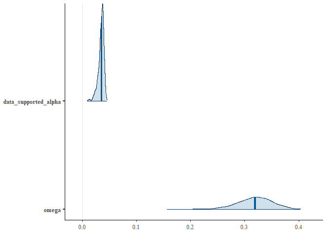
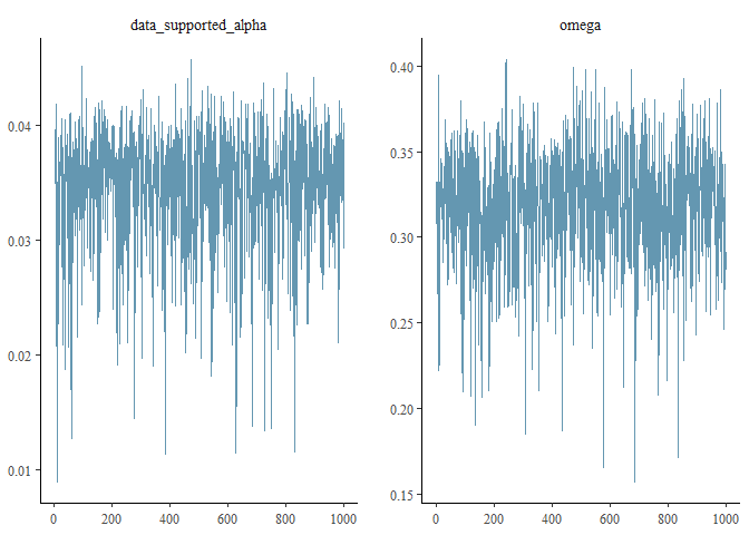
Packages such as bayesplot can be used to validate the model since it is built using rstan. For example, one may plot the marginal posterior distributions of the supported 210Pb activity and the memory parameter ;:
# load the bayesplot package
library("bayesplot")

# extract the parameters from the d_fit
d_parameters <- as.data.frame(rstan::extract(d_fit))

# plot of marginal posterior distribution
bayesplot::mcmc_areas(d_parameters,
                      pars = c("data_supported_alpha", "omega"),
                      prob = 0.99)
... or a trace plot of these parameters:
bayesplot::mcmc_trace(d_parameters,
                      pars = c("data_supported_alpha", "omega"))
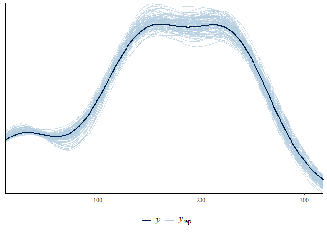
... or make a posterior predictive check for the model:
# load package stringr (just to construct an index for the predicted values in d_parameters)
library(stringr)

# define an index for predicted values in d_parameters
d_predicted_index <- stringr::str_detect(colnames(d_parameters), "^p_tot\\.")

# plot the posterior predictive check
bayesplot::ppc_dens_overlay(y = d_model$stan_data$data_chronology_y,
                 yrep = as.matrix(d_parameters[1:100, d_predicted_index])) +
  theme(legend.position = "bottom")
The manual contains more information on the functions and important things to consider during Bayesian analysis, such as the choice of prior parameters.
plumstan estimates the age of sediment layers (age-depth model) based on measured depth profiles of 210Pb activities, needing measured 210Pb activities and the corresponding measurement errors as input and yielding a posterior probability distribution (PPD) of the age of each depth section.
plumstan uses for this the statistical framework developed by Aquino-López et al (2018) that is inspired by the statistical framework of the popular software package for 14C dating, Bacon (Blaauw and Christen 2011).
The age-depth profile is modeled conditional on (1) the decay of 210Pb in the sediment leading to the measured 210Pb activity profile and (2) a sediment accumulation model.
The sediment accumulation model models the sediment accumulation [yr cm-1] for artificially constructed sections with a fixed thickness. Sections are constructed from the surface (depth = 0 cm) until the deepest depth of the measured profile (Aquino-López et al. 2018).
The thickness can be specified manually. Increasing the thickness results in fewer sections and thus a less smooth representation of the age depth profile.
Key features of the sediment accumulation model are that sediment accumulation rate is ≥ 0, and the sediment accumulation rate of a constructed section depends on the sediment accumulation of the next deeper section. The strength of this dependency is estimated by the model, ranging from 0 (the sediment accumulation rates of subsequent sections are independent) to 1 (the sediment accumulation rates of subsequent sections are identical). These features lead to realistic constraints for estimated sediment accumulation rates (Aquino-López et al. 2018, Blaauw and Christen (2011)).
Please cite this software package as:
Henning Teickner, (2020). plumstan: Bayesian 210Pb dating with Stan. Accessed 23 Apr 2020. Online at https://github.com/henningte/plumstan.
Text and figures : CC-BY-4.0
Code : See the DESCRIPTION file
Data : CC-BY-4.0 (see sources section for data sources and how to give credit to the original author(s) and the source)
We welcome contributions from everyone. Before you get started, please see our contributor guidelines. Please note that this project is released with a Contributor Code of Conduct. By participating in this project you agree to abide by its terms.
The complete data is derived from Aquino-López et al (2018) and was restructured to match the requirements of plumstan. The original article containing the data can be downloaded from https://link.springer.com/article/10.1007%2Fs13253-018-0328-7 and is distributed under the Creative Commons Attribution 4.0 International License (http://creativecommons.org/licenses/by/4.0/).
Aquino-López, Marco A., Maarten Blaauw, J. Andrés Christen, and Nicole K. Sanderson. 2018. “Bayesian Analysis of
Blaauw, Maarten, and J. Andrés Christen. 2011. “Flexible Paleoclimate Age-Depth Models Using an Autoregressive Gamma Process.” Bayesian Analysis 6 (3): 457–74. doi:10.1214/11-BA618.
Carpenter, Bob, Andrew Gelman, Matthew D. Hoffman, Daniel Lee, Ben Goodrich, Michael Betancourt, Marcus Brubaker, Jiqiang Guo, Peter Li, and Allen Riddell. 2017. “Stan : A Probabilistic Programming Language.” Journal of Statistical Software 76 (1). doi:10.18637/jss.v076.i01.
Stan Development Team. 2019. “RStan: The R Interface to Stan.” https://mc-stan.org.
