helonin / Feet_U-Net

Feet U-Net

Semantic segmentation of thermal feet images for characterizing epidural anesthesia performance during birth using a modified U-Net neural network.

Google Colab demo:

GUI project: https://github.com/blotero/FEET-GUI

Dataset

The used dataset contains images from 22 different patients. Each patient has between 6 and 18 images. There are 196 thermographic images in total, from which 157 were used to train the model and 39 to test it.

Results

Training History

Metrics:

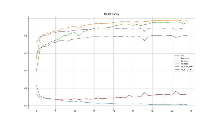
Different metrics on the test set

Segmentation	Dice	Jaccard (IoU)	Specificity	Sensitivity	Precision
U-Net	89.33 ± 6.07	81.24 ± 9.46	98.15 ± 1.83	90.65 ± 6.09	88.93 ± 9.73
U-Net + Post-processing	89.96 ± 5.77	82.22 ± 9.0	98.41 ± 1.56	90.53 ± 6.19	90.16 ± 8.88

The Post-processing step is explained down below in the Predict section.

Confusion Matrix

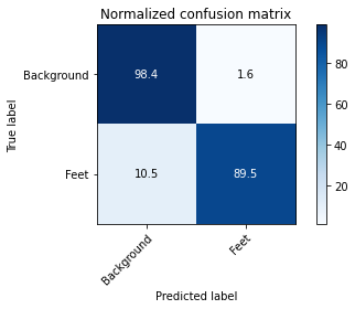
This confusion matrix was built using all the images of the test set.

Usage

1. Clone the repository

$ git clone https://github.com/Rmejiaz/Feet_U-Net

2. Install the requirements

$ pip install -r requirements.txt

From now on, it is easier to work directly on the directory U-Net:

$ cd U-Net

3. Download the dataset

It is possible to download the feet dataset in google colab, kaggle, or a linux machine executing the script download_dataset.py as follows:

$ python download_dataset.py --path=DOWNLOAD PATH

The download path is relative to the current directory, if left unspecified it will download the dataset to the current working direcory.

(Optional) Data Augmentation

It is possible to do data augmentation to the images and the masks using the script augmentation.py. It applies some random transformations to the input images such as rotations, crops and shiftings.

$ python augmentation.py --img_path=PATH TO IMAGES DIRECTORY --masks_path=PATH TO MASKS DIRECTORY --augmented_path=PATH TO SAVE THE NEW DATASET --labels=PATH OF THE LABELMAP n_images=NUMBER OF IMAGES TO GENERATE 

It will automatically create a new dataset in the specified path. If left unspecified, it creates the new dataset in the current working directory. By default, img_path = ./Dataset_Unificado/Train/Processed_Images , masks_path = ./Dataset_Unificado/Train/BinaryMasks , labels = ./Dataset_Unificado/binary_labelmap.txt and n_images = 192

(It is advided to be used with caution, as results do not necessarily improve when a large number of images are generated)

4. Train

In order to train the model, run the following command:

$ python train.py --imgs_path=PATH TO IMAGES DIRECTORY --masks_path=PATH TO MASKS DIRECTORY --val_imgs=PATH TO THE IMAGES FOR VALIDATION --val_masks=PATH TO THE MASKS FOR VALIDATION --val_split=VALIDATION SPLIT --weights=PATH TO SAVE THE TRAINED WEIGHTS --buffer_size=BUFFER_SIZE --batch_size=BATCH SIZE --epochs=NUMBER OF EPOCHOS --save_freq=SAVE FREQUENCY FOR THE CHECKPOINTS --save_model=PATH TO SAVE THE MODEL (.h5 FORMAT)

If val_split is set to 0, val_imgs and val_masks will be used for validation. Otherwise, it will split the training dataset according to val_split and use it for validation.

The defaults are: imgs_path=./Dataset_CVAT2/JPEGImages/Train , masks_path=./Dataset_CVAT2/SegmentationClass/Train val_imgs = ./Dataset_CVAT2/JPEGImages/Test , val_masks = ./Dataset_CVAT2/SegmentationClass/Test , weights = ./weights/ , buffer_size = 100 , batch_size = 5 , epochs = 10 , save_freq = 5

The weights will be saved to weights and the training history will also be saved in ./results/history0. The complete model will be saved in the specified directory in save_model. By default it will be saved to ./results/Model.h5

5. Predict

Do a prediction using trained weights or model.

$ python predict.py --image_path=IMAGE PATH --mask_path=MASK PATH --labels=LABELS PATH --show_results=True --model_path=WEIGHTS OR MODEL PATH --clean_prediction=WHETER TO CLEAN THE PREDICITON OR NOT

The defaults for the different arguments are the same ones as used before

It is possible to make a prediction using weights or directly a model in .h5 format. By default, model_path is set to ./results/Model.h5 (both .h5 and .ckpt formats are supported)

By default, the prediction is passed through a post-processing process, which removes all objects with sized below a defined threshold. This is done using the cv2 function connectedComponentsWithStats. It is also possible to obtain the pure prediction by setting clean_prediction to False

6. Evaluate

Make a prediction for a test set and measure dice and jaccard scores

$ python evaluate.py --model_path=MODEL PATH --test_images=IMAGES DIRECTORY PATH --test_masks=MASKS DIRECTORY PATH --results=PATH TO SAVE THE RESULTS

By default, test_images and test_masks are set to ./Dataset_CVAT2/JPEGImages/Test and ./Dataset_CVAT2/SegmentationClass/Test. and restuls to ./restults/. model_path supports both .ckpt files (weights) and .h5 complete trained model.

After running the script, a figure containing the Dice and Jaccard scores boxplot for the test images is generated and saved in results, as well as a subdirectory containing the predictions of the test set.

Download and use a pre-trained model

Download link: https://drive.google.com/file/d/1S-pUZZONC3fqMSvXfBg_7tGdxtkLIs-F/view?usp=sharing

It is also possible to download a pretrained model, which can be later used to make predictions as follows:

model = tf.keras.models.load_model('Model1.h5')

Y_pred = model.predict(X)

Or using predict.py, as shown before.

This model achieved very similar results to those shown on the Results

TO DO

Segmentation:

• U-Net implementation to segment feet and background.
• U-Net implementation to segment the differentes parts of the foot.
• Create a toy dataset to compare the performance.
• Data augmentation
• Re-label the dataset (optional)
• Improve Dice to at least 80%.
• Closing and Opening