RNA velocity is a computational method used in single-cell transcriptomics to predict the future state of individual cells based on their current gene expression profiles. It provides insights into the direction and speed of changes in gene expression, effectively estimating how cells are transitioning between different cellular states over time.
The name "velocity" comes from its conceptual analogy with classical physics. In physics, velocity is a measure of the rate of change of an object's position with respect to time. Similarly, in the context of single-cell transcriptomics, RNA velocity aims to estimate the rate at which the gene expression profile of a cell changes over time. This can help researchers understand the dynamics of cellular processes, such as differentiation, activation, or response to stimuli.
So, the goal is to gain insights into the dynamics of gene expression changes in individual cells over time. This analysis provides information about the rate and direction of changes in gene expression, allowing researchers to infer the future states of individual cells and identify cellular transitions and trajectories.
ScRNA velocity analysis relies on the measurement of the ratio between unspliced and spliced mRNA molecules within a cell. Such data can be stored in a loom format file. A loom file is a kind of specialized HDF5 file type designed to store large matrices such as count tables and their accompanying metadata. In a loom file, there can be three count tables for a single sample: spliced transcripts, unspliced transcripts, and ambiguous transcripts.
By quantifying the abundance of these RNA species, it is possible to infer the directionality and speed of gene expression changes, providing valuable information about cell fate decisions, differentiation processes, and developmental trajectories.
In this notebook, we accomplish the following:
To calculate basic velocity parameters
To fit a dynamical model that can capture the dynamic of transcriptome more effectively
To adjust for the effect of having more than one lineage of cells in the datasetss
#import libs
import os
import scvelo as scv
import pandas as pd
import scanpy as sc
import anndata
import numpy as np
import matplotlib.pyplot as plt
import statsmodels.graphics.mosaicplot as mplt
import rpy2.robjects as robjects
import warnings
print(f"scvelo version: {scv.__version__}")
print(f"scanpy version: {sc.__version__}")
print(f"numpy version: {np.__version__}")
print(f"pandas version: {pd.__version__}")
scvelo version: 0.2.5
scanpy version: 1.9.3
numpy version: 1.21.6
pandas version: 1.3.5
# Setting scvelo parameters
# Needed to run R magic
%load_ext rpy2.ipython


scv.settings.verbosity = 3  # show errors(0), warnings(1), info(2), hints(3)
scv.settings.presenter_view = True  # set max width size for presenter view
scv.settings.set_figure_params('scvelo')  # for beautified visualization

# Ignore all deprecation warnings
warnings.filterwarnings("ignore", category=DeprecationWarning)%%R
library(Seurat)
epi <- readRDS("updated_epi_seurat.RDS")
epi2= %R epi%%R
# To extract UMAP coordinates
umap <- Embeddings(epi, reduction = "umap")
write.csv(umap, file = "cell_embeddings.csv")
# To extract clusters
metadata <- epi@meta.data
write.csv(metadata, file = "metadata.csv")
# To extract cells
cellID_obs <- as.data.frame(epi@meta.data$cells)
write.csv(cellID_obs, file = "cellID_obs.csv")
#"0" = "basal_cell",
#"1" = "cancer_associated_luminal_cell",
#"2" = "differentiated_luminal_cell",
#"3" = "unique_luminal_cell",
#"4" = "immunomodulatory_luminal_cell",
##"5" = "adhesion_signaling_luminal_cell"# transfer the variable to the Python namespace
cellID_obs = %R cellID_obs
umap = %R umap
metadata = %R metadatacellID_obs.rename(columns={"epi@meta.data$cells": "cells"}, inplace=True)cellID_obs["cells"].valuesarray(['SRR12603782:AAACCTGAGATGGGTCx', 'SRR12603782:AAACCTGAGCGATTCTx',
'SRR12603782:AAACCTGAGTGAAGTTx', ...,
'SRR12603790:TTTGTCAAGAAGGTGAx', 'SRR12603790:TTTGTCAGTTACAGAAx',
'SRR12603790:TTTGTCAGTTTCGCTCx'], dtype=object)
# Directory containing the loom files
loom_directory = "loom_files"

# List of cancer sample names
sample_names = ["SRR12603782", "SRR12603783", "SRR12603784", "SRR12603785", "SRR12603786", "SRR12603787", "SRR12603789", "SRR12603790"]

# Initialize a list to hold the filtered objects
filtered_samples = []

# Loop through each sample
for sample_name in sample_names:
    print(f"Processing sample: {sample_name}")

    # Read the loom file
    sample = anndata.read_loom(os.path.join(loom_directory, f"{sample_name}.loom"))

    # Filter based on cell IDs
    filtered_sample = sample[sample.obs_names.isin(cellID_obs.cells.tolist())]


    # Append the filtered object to the list
    filtered_samples.append(filtered_sample)
Processing sample: SRR12603782
Processing sample: SRR12603783
Processing sample: SRR12603784
Processing sample: SRR12603785
Processing sample: SRR12603786
Processing sample: SRR12603787
Processing sample: SRR12603789
Processing sample: SRR12603790
# Concotenating objects:

#First for each element in filtered_samples, make var names unique
for filtered_sample in filtered_samples:
    filtered_sample.var_names_make_unique()

#
epi_anndata = sc.concat(filtered_samples, axis = 0, join = 'outer')
# To check if all cells are present in the merged file
#List of cells you have
list_of_cells = cellID_obs.cells.tolist()
# Check if all cells in merged anndata are present in the list
all_cells_present = all(cell in list_of_cells for cell in epi_anndata.obs_names)
if all_cells_present:
print("All cells in the merged anndata are present in the list.")
else:
print("Not all cells in the merged anndata are present in the list.")All cells in the merged anndata are present in the list.
saving cell ids ad a dataframe to later order them considering umap file
epi_anndata_index = pd.DataFrame(epi_anndata.obs.index)
epi_anndata_index = epi_anndata_index.rename(columns = {0:'Cell ID'})
umap = pd.read_csv("cell_embeddings.csv")
umap = umap.rename(columns = {'Unnamed: 0':'CellID'})
# Make cell ids comparable between
umap['CellID'] = umap['CellID'].str.replace('_', ':').str[:-2] + 'x'merging the index dataframe with UMAP, so the order will match our anndata object.
umap_ordered = epi_anndata_index.merge(umap, on = "CellID")Since we're certain the orders are the same, we can remove the first column of the data frame and add the UMAP coordinates to our anndata object.
umap_ordered = umap_ordered.iloc[:,1:]
epi_anndata.obsm['X_umap'] = umap_ordered.values
# Adding clusters and the rest of metadata
# Modify the index (row names)
metadata.rename(columns={'cells': 'CellID'}, inplace=True)
new_index = [name.replace('_', ':').replace('-1', 'x') for name in metadata.index]
metadata.index = new_index
#metadata
metadata_ordered = epi_anndata_index.merge(metadata, on = "CellID")
# set index
metadata_ordered.set_index('CellID', inplace=True)
metadata_ordered.index.name = None# Assign the old metadata to the anndata
epi_anndata.obs = metadata_ordered
# convert clusters column to categorical column
epi_anndata.obs['clusters'] = epi_anndata.obs['clusters'].astype(str)
#obs_vals.cat.categories = obs_vals.cat.categories.astype(str).tolist()
#epi_anndata.obs['clusters'] = epi_anndata.obs['clusters'].astype('category')
# Setting colors based on clsuter colors from Seurat
clusters_colors = ["#A6CEE3","#2E81B9", "#B2DF8A", "#33A02C", "#FDBF6F", "#FF7F00"]
# Adding cluster colors to the anndata object
epi_anndata.uns['clusters_colors'] = clusters_colorsepi_anndata.write('scvelo_epi.h5ad', compression='gzip')NB This section is adapted from Differential Kinetics tutorial from scvelo documentation
One important concern is dealing with systems that represent multiple lineages and processes, where genes are likely to show different kinetic regimes across subpopulations. Distinct cell states and lineages are typically governed by different variations in the gene regulatory networks and may hence exhibit different splicing kinetics. This gives rise to genes that display multiple trajectories in phase space.
To address this, the dynamical model can be used to perform a likelihood-ratio test for differential kinetics. This way, we can detect clusters that display kinetic behavior that cannot be well explained by a single model of the overall dynamics. Clustering cell types into their different kinetic regimes then allows fitting each regime separately.
Processing consists of gene selection, log-normalizing, and computing moments. See the previous tutorials for further explanation.
adata = scv.read('scvelo_epi.h5ad')
# matching color to the cluster colors in Seurat object with Slingshot data
adata.uns['clusters_colors'] = ["#FF7F00", "#A6CEE3","#2E81B9", "#B2DF8A", "#FDBF6F","#33A02C"]adata.obs['clusters'].value_counts()basal_cell 6388
cancer_associated_luminal_cell 5424
differentiated_luminal_cell 3782
unique_luminal_cell 3674
immunomodulatory_luminal_cell 3593
adhesion_signaling_luminal_cell 1999
Name: clusters, dtype: int64
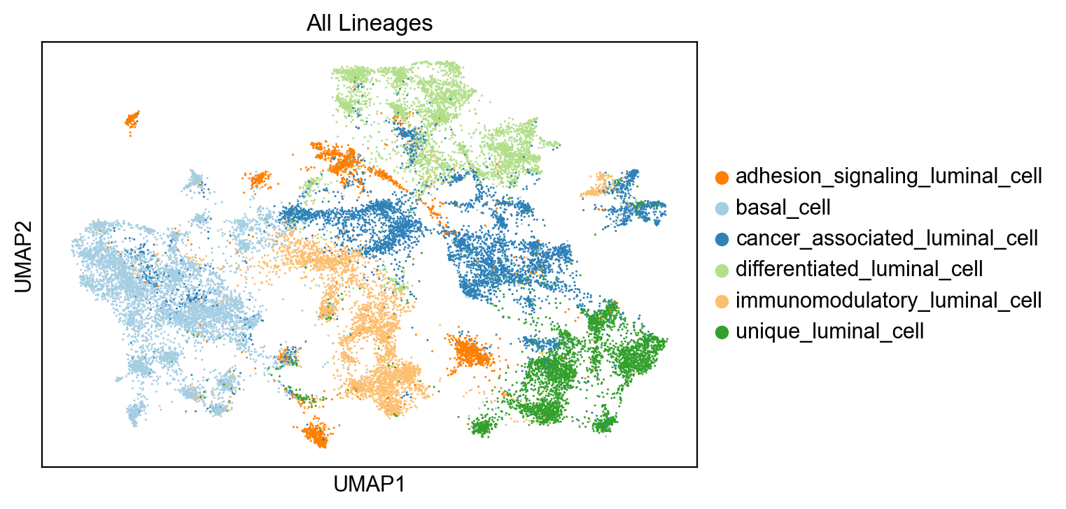
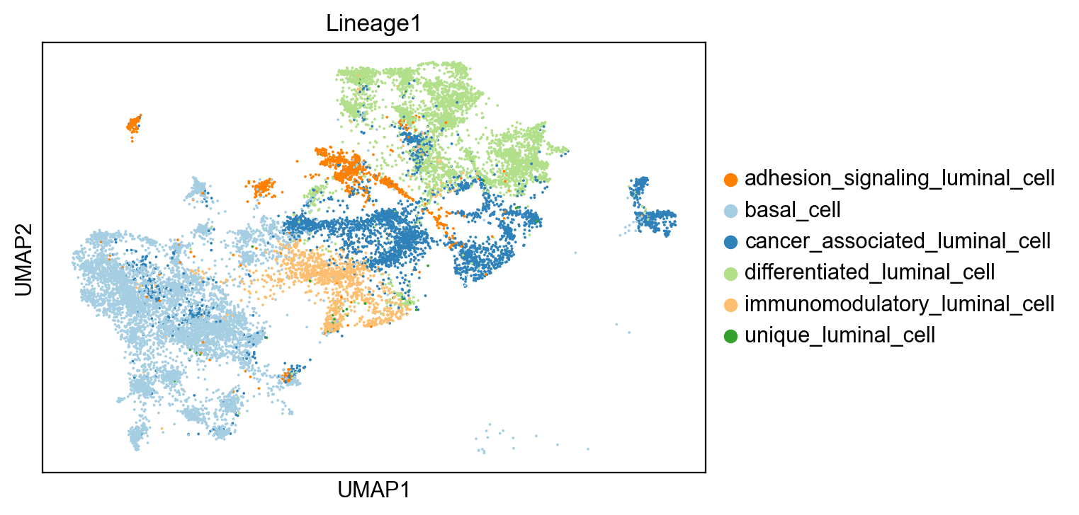
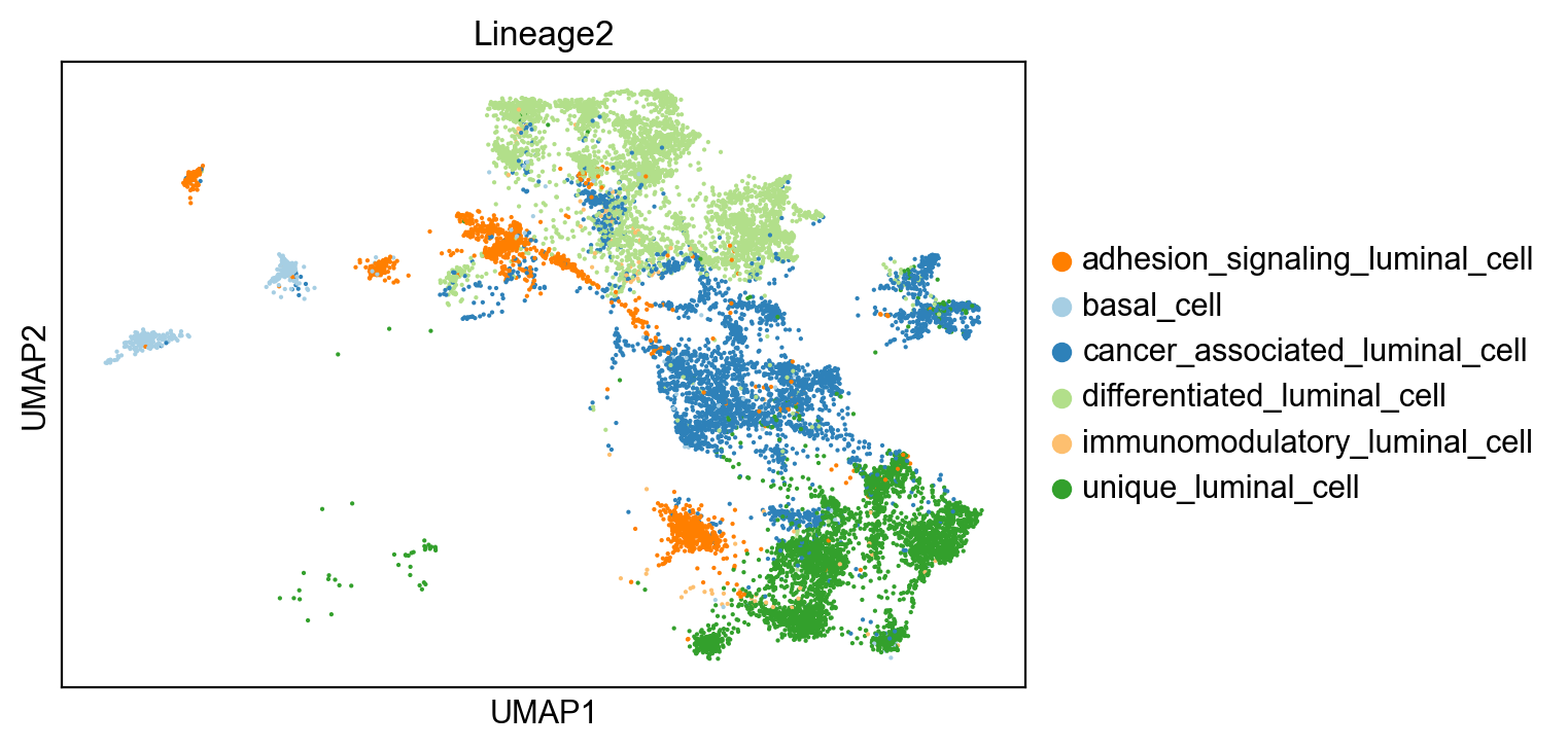
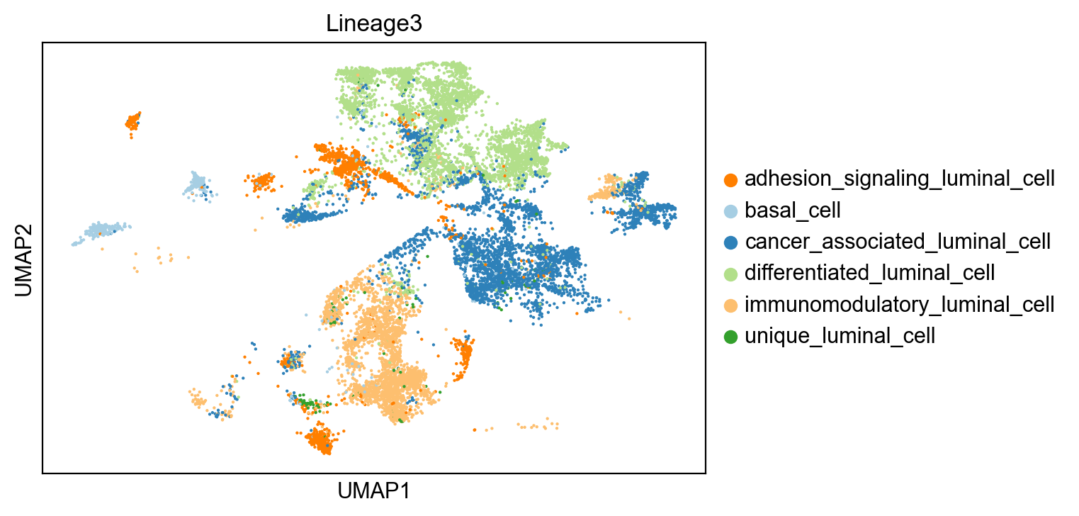
Earlier in RNA trajectory inference, we used slingshot and identified three lineages in our dataset. Here, we will be focusing only on Lineage 1, as it includes cells showing a transition from basal cells to differentiated luminal cells to cancer-associated luminal cells to immunomodulatory cancer luminal cells to cancer basal cells.
scv.pp.filter_and_normalize(adata, min_shared_counts=30, n_top_genes=2000)Filtered out 26467 genes that are detected 30 counts (shared).
Normalized count data: X, spliced, unspliced.
Extracted 2000 highly variable genes.
Logarithmized X.
sc.pl.umap(adata, color= 'clusters', title='All Lineages')
sc.pl.umap(adata[~adata.obs['Lineage1'].isna()], color= 'clusters', title='Lineage1')
sc.pl.umap(adata[~adata.obs['Lineage2'].isna()], color= 'clusters', title='Lineage2')
sc.pl.umap(adata[~adata.obs['Lineage3'].isna()], color= 'clusters', title='Lineage3')
C:\Users\User1\anaconda3\envs\scVelo\lib\site-packages\scanpy\plotting\_tools\scatterplots.py:163: MatplotlibDeprecationWarning: The get_cmap function was deprecated in Matplotlib 3.7 and will be removed two minor releases later. Use ``matplotlib.colormaps[name]`` or ``matplotlib.colormaps.get_cmap(obj)`` instead.
cmap = copy(get_cmap(cmap))
print("cells in Lineage1")
print()
print(adata[~adata.obs['Lineage1'].isna()].obs['clusters'].value_counts())
print()
print("cells in Lineage2")
print()
print(adata[~adata.obs['Lineage2'].isna()].obs['clusters'].value_counts())
print()
print("cells in Lineage3")
print()
print(adata[~adata.obs['Lineage3'].isna()].obs['clusters'].value_counts())
cells in Lineage1
basal_cell 6322
differentiated_luminal_cell 3734
cancer_associated_luminal_cell 3570
immunomodulatory_luminal_cell 1271
adhesion_signaling_luminal_cell 1100
unique_luminal_cell 41
Name: clusters, dtype: int64
cells in Lineage2
differentiated_luminal_cell 3671
cancer_associated_luminal_cell 3590
unique_luminal_cell 3563
adhesion_signaling_luminal_cell 1548
basal_cell 431
immunomodulatory_luminal_cell 105
Name: clusters, dtype: int64
cells in Lineage3
cancer_associated_luminal_cell 3812
differentiated_luminal_cell 3743
immunomodulatory_luminal_cell 2781
adhesion_signaling_luminal_cell 1575
basal_cell 483
unique_luminal_cell 135
Name: clusters, dtype: int64
# Selecting Lineage
adata = adata[~adata.obs['Lineage1'].isna()]We need the first and second order moments (means and uncentered variances) computed among nearest neighbors in PCA space, summarized in scv.pp.moments, which internally computes scv.pp.pca and scv.pp.neighbors. First order is needed for deterministic velocity estimation, while stochastic estimation also requires second order moments.
scv.pp.moments(adata, n_pcs=30, n_neighbors=30)computing neighbors
finished (0:00:14) --> added
'distances' and 'connectivities', weighted adjacency matrices (adata.obsp)
computing moments based on connectivities
finished (0:00:01) --> added
'Ms' and 'Mu', moments of un/spliced abundances (adata.layers)
Velocity analysis in gene expression space involves calculating vectors representing cell movement direction and speed. Velocities are derived by modeling mRNA dynamics, either probabilistically (stochastic mode) , with certainty (deterministic mode) or dynamic mode. Genes' pre-mature and mature mRNA ratios yield constant transcriptional states, with positive velocities indicating up-regulation due to higher unspliced mRNA, and negative velocities suggesting down-regulation. A dynamic mode requires prior execution of scv.tl.recover_dynamics(adata). Transition probabilities of cell-to-cell shifts are estimated using cosine correlation and stored in a velocity graph matrix. Converting this graph into a transition matrix involves applying a Gaussian kernel. The velocity graph also aids in projecting velocities into lower-dimensional spaces, enabling trajectory analysis and identifying terminal states through cellular transitions.
scv.tl.velocity(adata)computing velocities
finished (0:00:02) --> added
'velocity', velocity vectors for each individual cell (adata.layers)
scv.tl.velocity_graph(adata, n_jobs=20)computing velocity graph (using 20/32 cores)
0%| | 0/16038 [00:00<?, ?cells/s]
finished (0:00:13) --> added
'velocity_graph', sparse matrix with cosine correlations (adata.uns)
#scv.pl.velocity_embedding_stream(adata, basis='umap', save= 'stream_plot.png')
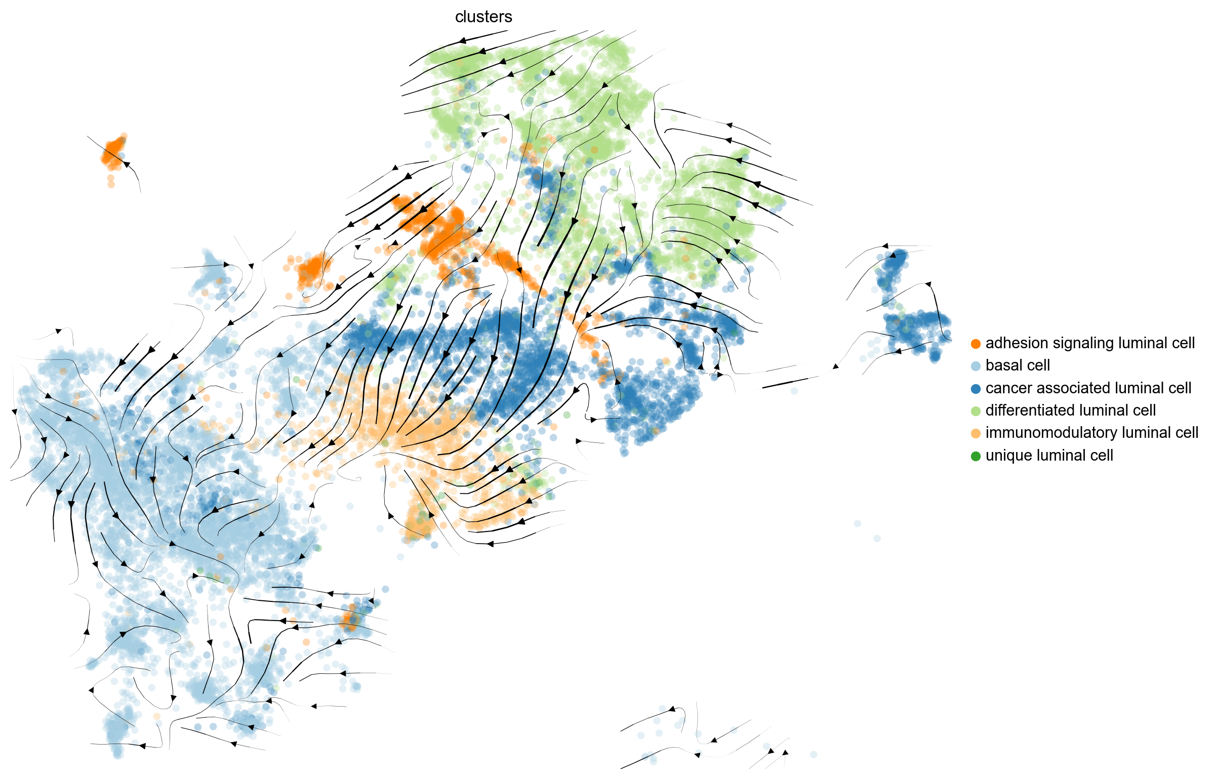
scv.pl.velocity_embedding_stream(adata, basis='umap', legend_loc='right margin', figsize=(10, 8),min_mass=0, save= 'stream_plot.png')
computing velocity embedding
finished (0:00:02) --> added
'velocity_umap', embedded velocity vectors (adata.obsm)
saving figure to file ./figures/scvelo_stream_plot.png
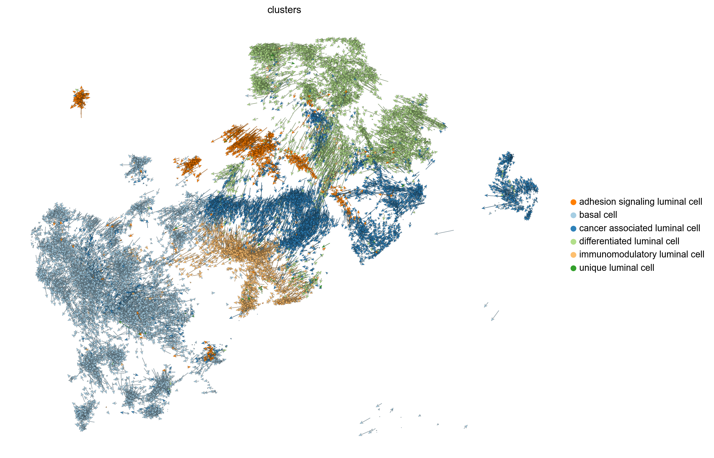
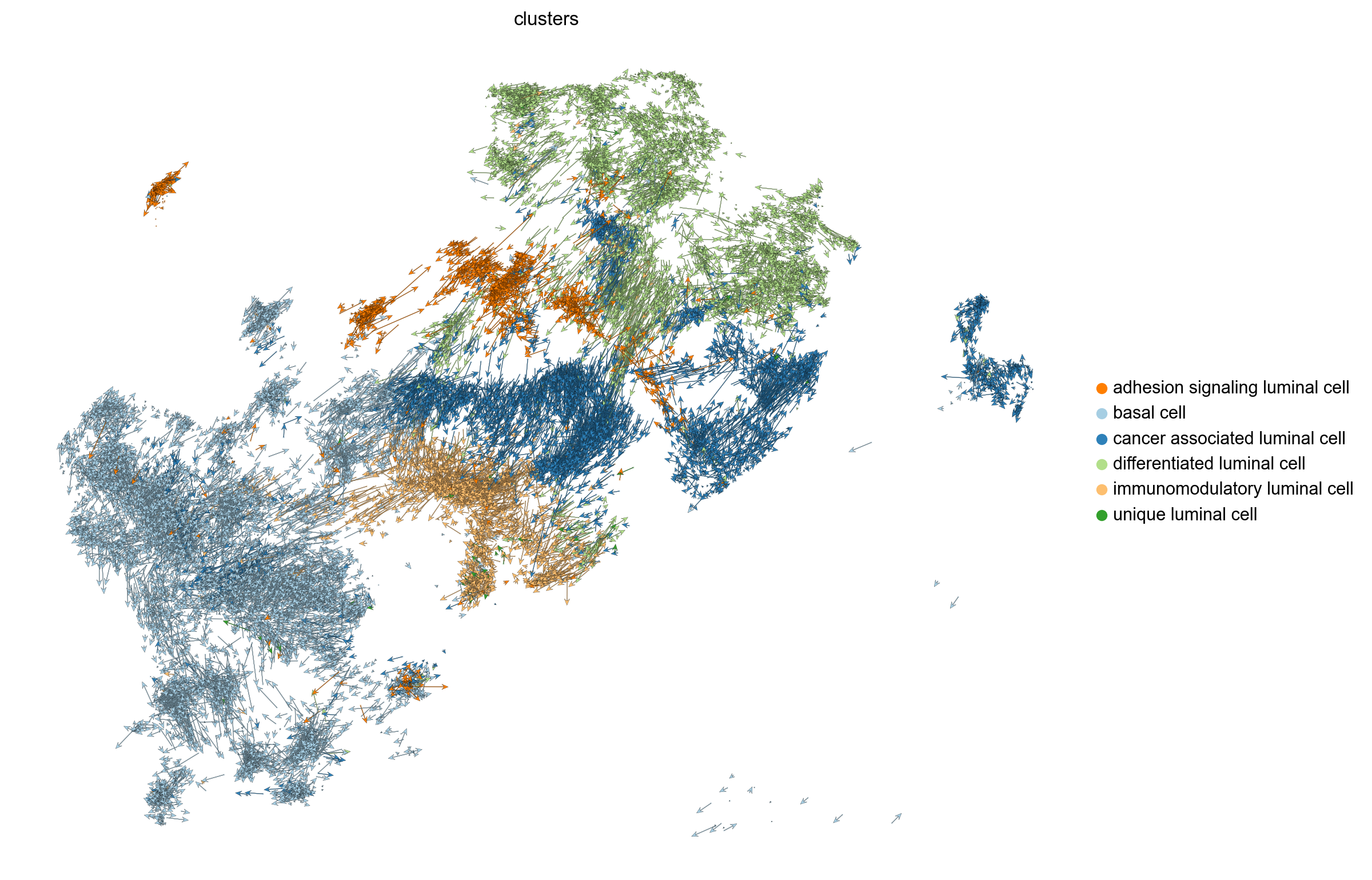
scv.pl.velocity_embedding(adata, basis='umap', legend_loc='right margin',arrow_length=8.0, figsize=(10, 8), save= 'embedding_plot.png')saving figure to file ./figures/scvelo_embedding_plot.png
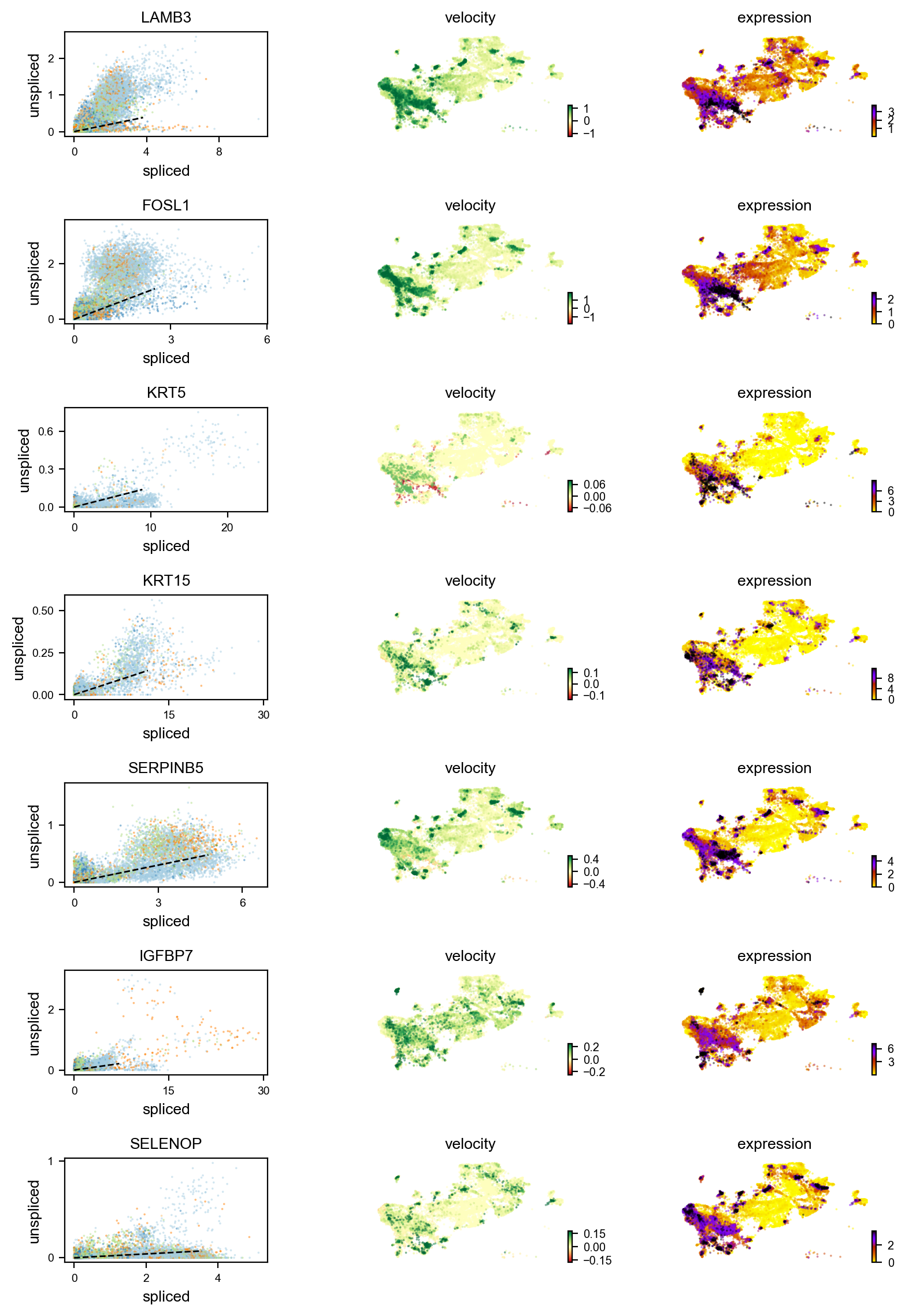
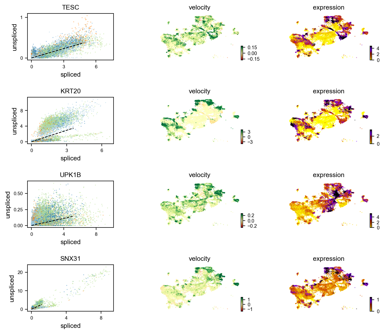
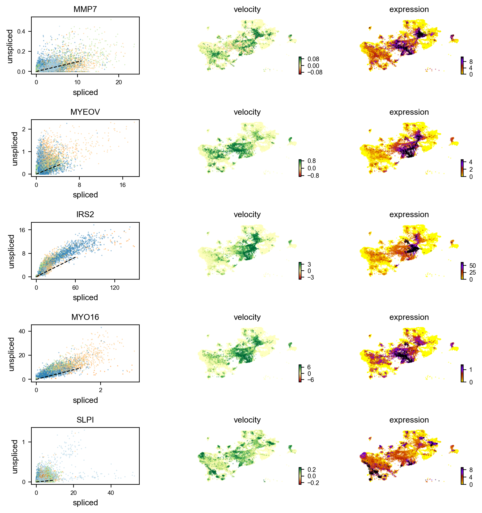
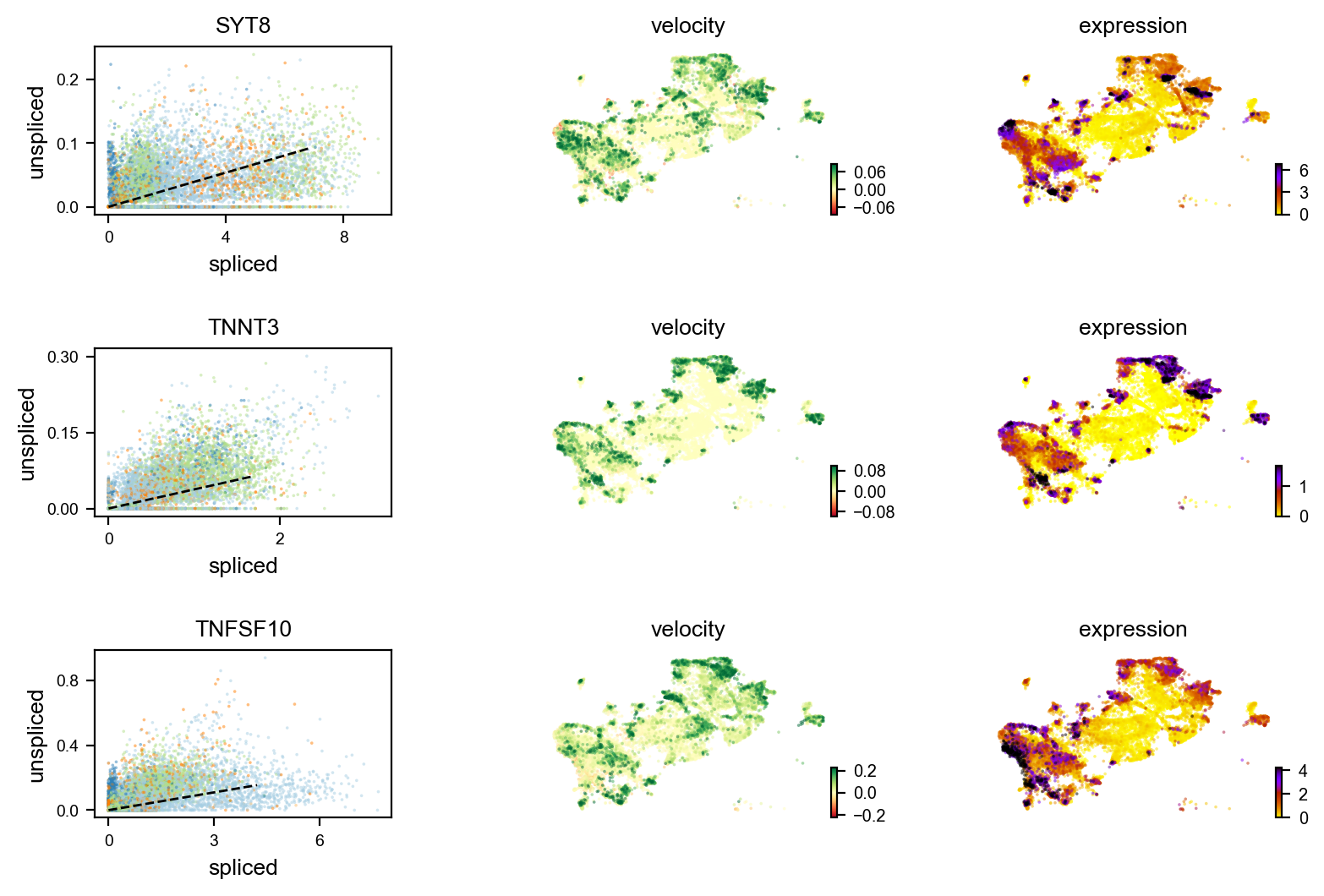
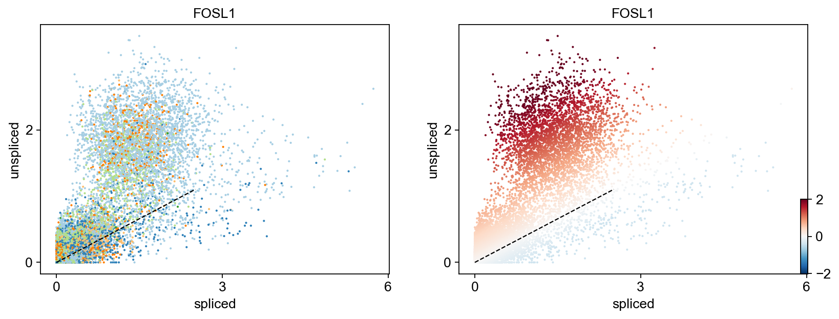
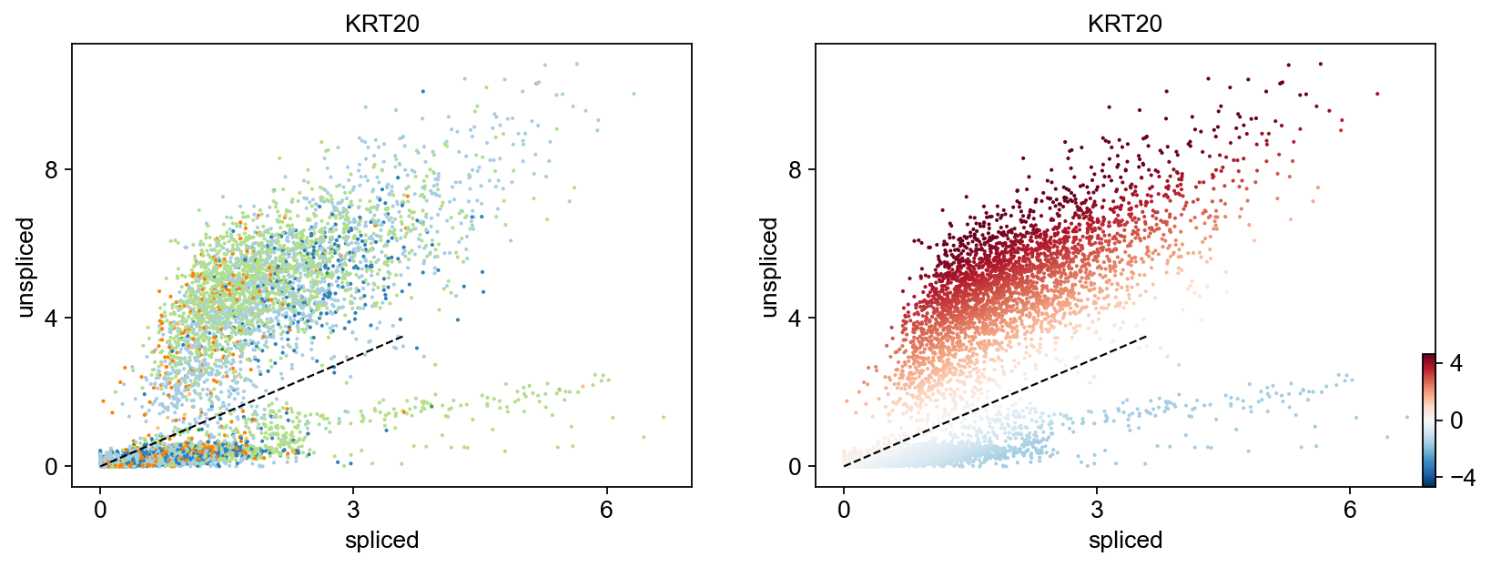
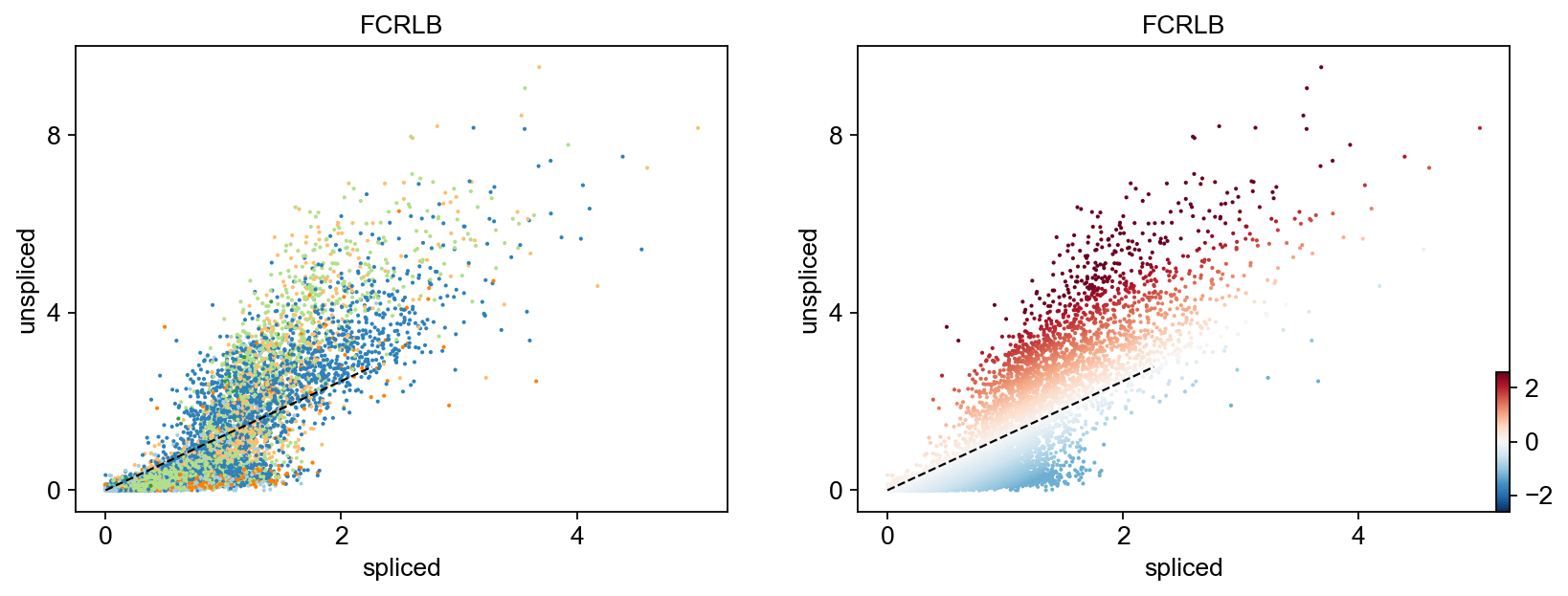
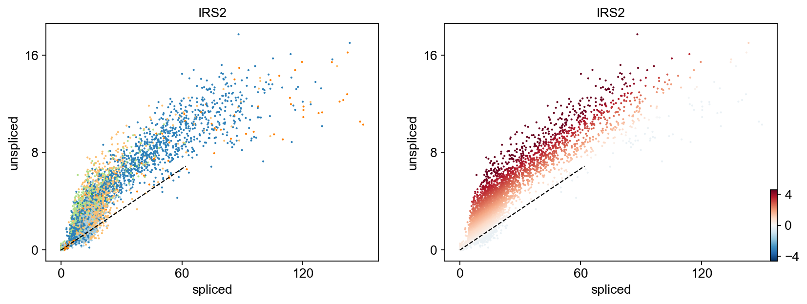
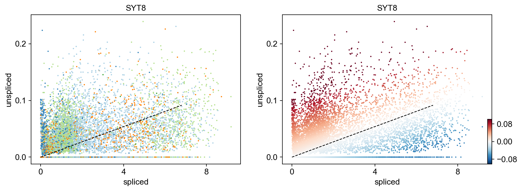
Gene activity is regulated by transcription. Induction leads to increased precursor unspliced mRNA, while repression results in decreased unspliced mRNA. Spliced mRNA is derived from unspliced mRNA with a time lag. Time is latent; hence, dynamics are deduced from measured spliced and unspliced mRNAs in the phase portrait. Let's visualize velocity for some marker genes in different clusters where they have been identified as velocity_gene. In the images below the black line corresponds to the estimated ‘steady-state’ ratio, i.e. the ratio of unspliced to spliced mRNA abundance which is in a constant transcriptional state. RNA velocity for a particular gene is determined as the residual, i.e. how much an observation deviates from that steady-state line. Positive velocity indicates that a gene is up-regulated, which occurs for cells that show higher abundance of unspliced mRNA for that gene than expected in steady state. Conversely, negative velocity indicates that a gene is down-regulated.
#For basal markers

basal_markers = ['KRT15','KRT5','BCAM','IGFBP2','IGFBP7','CDH13','FOSL1','LAMB3','COL4A5','SERPINB5','SELENOP']
velocity_basal_markers=adata.var.index[adata.var.index.isin(basal_markers) & adata.var['velocity_genes']==True]
scv.pl.velocity(adata, velocity_basal_markers)
C:\Users\User1\anaconda3\envs\scVelo\lib\site-packages\scvelo\plotting\utils.py:869: MatplotlibDeprecationWarning: The draw_all function was deprecated in Matplotlib 3.6 and will be removed two minor releases later. Use fig.draw_without_rendering() instead.
cb.draw_all()
#For luminal differentiated
markers = ['NDUFA4L2','CRH','UPK2','SNX31','KRT20','AC019117.2','UPK1B','LINC02163','H19','TESC']
velocity_diffLum_markers=adata.var.index[adata.var.index.isin(markers) & adata.var['velocity_genes']==True]
scv.pl.velocity(adata, velocity_diffLum_markers)#For cancer-associated luminal cells
markers = ['UCA1','LGALS1','CA9','SPINK1','GJB2','PTPRR','FCRLB','PLA2G2F','GJB6','FBLN1']
velocity_diffLum_markers=adata.var.index[adata.var.index.isin(markers) & adata.var['velocity_genes']==True]
scv.pl.velocity(adata, velocity_diffLum_markers)#For immunomodulatory luminal cells
markers = ['S100A9','C15orf48','MYO16','MMP7','MYEOV','AC025159.1','LTO1','IFI27','IRS2','SLPI']
velocity_diffLum_markers=adata.var.index[adata.var.index.isin(markers) & adata.var['velocity_genes']==True]
scv.pl.velocity(adata, velocity_diffLum_markers)#For unique luminal cells
markers = ['LY6D','TNNT3','IGF2BP2','GMNN','SYT8','AC068587.4','ITM2C','SGPP2','ZNF750','TNFSF10']
velocity_diffLum_markers=adata.var.index[adata.var.index.isin(markers) & adata.var['velocity_genes']==True]
scv.pl.velocity(adata, velocity_diffLum_markers)# visualization for select genes with distinct velocity pattern
for gene in ['FOSL1', 'KRT20', 'FCRLB', 'IRS2','SYT8']:
scv.pl.scatter(adata,gene , color=['clusters', 'velocity'])To systematically, identify genes that may help explain the resulting vector field and inferred lineages, we can test which genes have cluster-specific differential velocity expression, being siginificantly higher/lower compared to the remaining population. The module scv.tl.rank_velocity_genes runs a differential velocity t-test and outpus a gene ranking for each cluster.
Thresholds can be set (e.g. min_corr) to restrict the test on a selection of gene candidates. The min_corr parameter sets a threshold for the minimum Spearman's correlation coefficient between spliced and unspliced counts that a gene needs to have to be considered in the ranking of velocity genes. This means that only genes with a correlation coefficient above this threshold will be included in the ranking analysis.
scv.tl.rank_velocity_genes(adata, groupby='clusters', min_corr=.5)
df = scv.DataFrame(adata.uns['rank_velocity_genes']['names'])
df.head()
#
df.to_csv("velocity_ranked_genes.csv")ranking velocity genes
C:\Users\User1\anaconda3\envs\scVelo\lib\site-packages\scvelo\tools\utils.py:501: DeprecationWarning: Please use `rankdata` from the `scipy.stats` namespace, the `scipy.stats.stats` namespace is deprecated.
from scipy.stats.stats import rankdata
finished (0:00:04) --> added
'rank_velocity_genes', sorted scores by group ids (adata.uns)
'spearmans_score', spearmans correlation scores (adata.var)
C:\Users\User1\AppData\Local\Temp\ipykernel_7140\713790817.py:3: DeprecationWarning: `scvelo.read_load.get_df` is deprecated since scVelo v0.2.4 and will be removed in a future version. Please use `scvelo.core.get_df` instead.
df = scv.DataFrame(adata.uns['rank_velocity_genes']['names'])
#For visualization:
kwargs = dict(frameon=False, size=10, linewidth=1.5)
scv.pl.scatter(adata, df['immunomodulatory_luminal_cell'][:5], ylabel='immuneLC', **kwargs)
scv.pl.scatter(adata, df['basal_cell'][:5], ylabel='basalCell', **kwargs)
scv.pl.scatter(adata, df['differentiated_luminal_cell'][:5], ylabel='diffLC', **kwargs)
scv.pl.scatter(adata, df['cancer_associated_luminal_cell'][:5], ylabel='cancerLC', **kwargs)
scv.pl.scatter(adata, df['unique_luminal_cell'][:5], ylabel='uniqueLC', **kwargs)The cell cycle detected by RNA velocity, could be biologically affirmed by cell cycle scores (standardized scores of mean expression levels of phase marker genes).
#scv.tl.score_genes_cell_cycle(adata)
#scv.pl.scatter(adata, color_gradients=['S_score', 'G2M_score'], smooth=True, perc=[10, 75])The previous module also computed a spearmans correlation score, which we can use to rank/sort the phase marker genes to then display their phase portraits.
#s_genes, g2m_genes = scv.utils.get_phase_marker_genes(adata)
#s_genes = scv.get_df(adata[:, s_genes], 'spearmans_score', sort_values=True).index
#g2m_genes = scv.get_df(adata[:, g2m_genes], 'spearmans_score', sort_values=True).index
#kwargs = dict(frameon=False, ylabel='cell cycle genes')
#scv.pl.scatter(adata, list(s_genes[:2]) + list(g2m_genes[:3]), **kwargs)Two more useful stats:
-
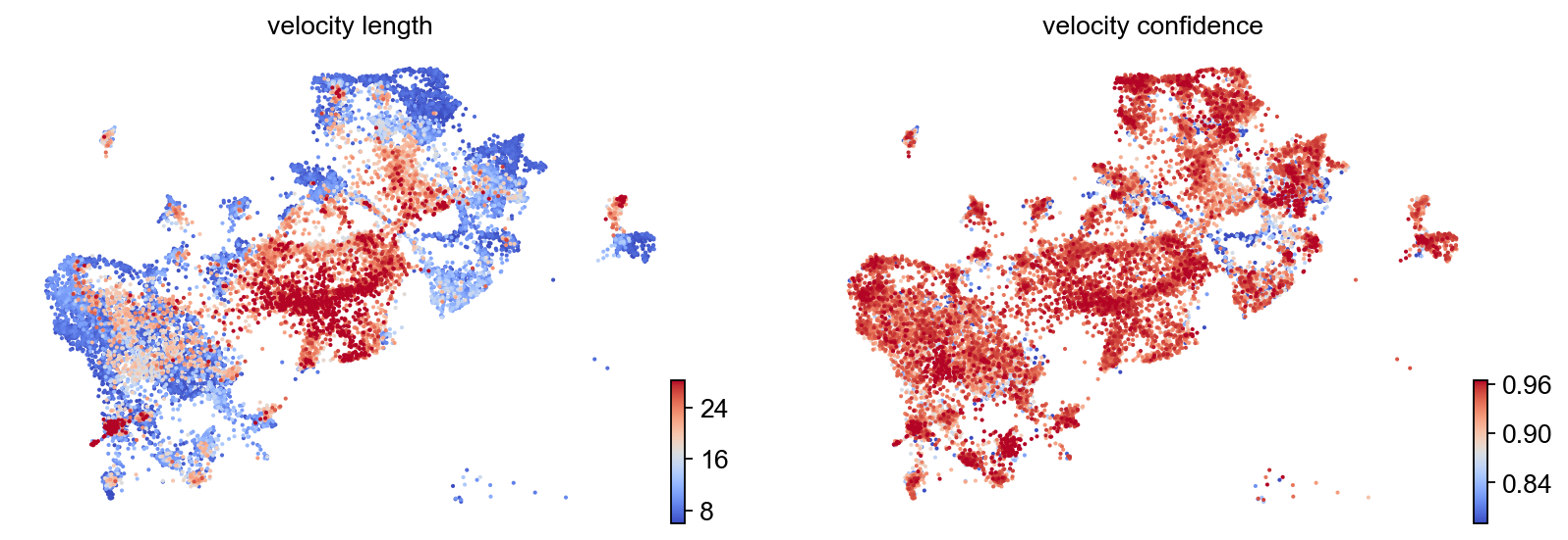
The speed or rate of differentiation is given by the length of the velocity vector.
-
The coherence of the vector field (i.e., how a velocity vector correlates with its neighboring velocities) provides a measure of confidence.
scv.tl.velocity_confidence(adata)
keys = 'velocity_length', 'velocity_confidence'
scv.pl.scatter(adata, c=keys, cmap='coolwarm', perc=[5, 95])--> added 'velocity_length' (adata.obs)
--> added 'velocity_confidence' (adata.obs)
--> added 'velocity_confidence_transition' (adata.obs)
C:\Users\User1\anaconda3\envs\scVelo\lib\site-packages\scvelo\plotting\utils.py:869: MatplotlibDeprecationWarning: The draw_all function was deprecated in Matplotlib 3.6 and will be removed two minor releases later. Use fig.draw_without_rendering() instead.
  cb.draw_all()
These provide insights where cells differentiate at a slower/faster pace, and where the direction is un-/determined.
On cluster-level, we find that differentiation speeds up for cancer_associated_luminal_cells and substantially increased in immunomodulatory_luminal_cell. In terms of the basal cells we can observe that diffrentitaion rate in some of the cells are low (normal basal cells?) and in some of them the rate is high (cancer basal cells?). The lowest level of diffrentiation rate belongs to differentiated luminal cells , which is expected.
df = adata.obs.groupby('clusters')[keys].mean().T
df.style.background_gradient(cmap='coolwarm', axis=1)
C:\Users\User1\anaconda3\envs\scVelo\lib\site-packages\pandas\io\formats\style.py:2818: MatplotlibDeprecationWarning: The get_cmap function was deprecated in Matplotlib 3.7 and will be removed two minor releases later. Use ``matplotlib.colormaps[name]`` or ``matplotlib.colormaps.get_cmap(obj)`` instead.
rgbas = plt.cm.get_cmap(cmap)(norm(gmap))
| clusters | adhesion_signaling_luminal_cell | basal_cell | cancer_associated_luminal_cell | differentiated_luminal_cell | immunomodulatory_luminal_cell | unique_luminal_cell |
|---|---|---|---|---|---|---|
| velocity_length | 11.031882 | 10.718401 | 17.621187 | 11.035123 | 25.891668 | 15.758536 |
| velocity_confidence | 0.859421 | 0.911380 | 0.913085 | 0.912155 | 0.940378 | 0.906360 |
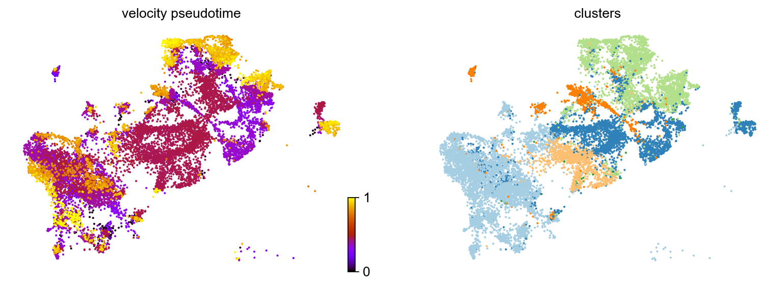
Based on the velocity graph, a velocity pseudotime can be computed. After inferring a distribution over root cells from the graph, it measures the average number of steps it takes to reach a cell after walking along the graph starting from the root cells. Contrarily to diffusion pseudotime, it implicitly infers the root cells and is based on the directed velocity graph instead of the similarity-based diffusion kernel.
scv.tl.velocity_pseudotime(adata)
#scv.pl.scatter(adata, color='velocity_pseudotime', cmap='gnuplot')
scv.pl.scatter(adata, color=['velocity_pseudotime', 'clusters'], cmap='gnuplot')
computing terminal states
identified 7 regions of root cells and 4 regions of end points .
finished (0:00:01) --> added
'root_cells', root cells of Markov diffusion process (adata.obs)
'end_points', end points of Markov diffusion process (adata.obs)
C:\Users\User1\anaconda3\envs\scVelo\lib\site-packages\scvelo\plotting\utils.py:869: MatplotlibDeprecationWarning: The draw_all function was deprecated in Matplotlib 3.6 and will be removed two minor releases later. Use fig.draw_without_rendering() instead.
cb.draw_all()
The bright yellow color indicates centers in the cancer associated luminal cells and basal cells where cells are newly diffrentiated. This can indicate existence of multiple lineages in the dataset
We run the dynamical model to learn the full transcriptional dynamics of splicing kinetics.
It is solved in a likelihood-based expectation-maximization framework, by iteratively estimating the parameters of reaction rates and latent cell-specific variables, i.e. transcriptional state and cell-internal latent time. It thereby aims to learn the unspliced/spliced phase trajectory for each gene.
scv.tl.recover_dynamics(adata, n_jobs=25)

scv.tl.velocity(adata, mode='dynamical')
scv.tl.velocity_graph(adata, n_jobs=25)
recovering dynamics (using 25/32 cores)
0%| | 0/698 [00:00<?, ?gene/s]
finished (0:01:51) --> added
'fit_pars', fitted parameters for splicing dynamics (adata.var)
computing velocities
finished (0:00:05) --> added
'velocity', velocity vectors for each individual cell (adata.layers)
computing velocity graph (using 25/32 cores)
0%| | 0/16038 [00:00<?, ?cells/s]
finished (0:00:06) --> added
'velocity_graph', sparse matrix with cosine correlations (adata.uns)
scv.pl.velocity_embedding_stream(adata, basis='umap', legend_loc='right margin', figsize=(10, 8), save= 'dynamical_stream_plot.png')computing velocity embedding
finished (0:00:02) --> added
'velocity_umap', embedded velocity vectors (adata.obsm)
saving figure to file ./figures/scvelo_dynamical_stream_plot.png
scv.pl.velocity_embedding(adata, basis='umap', legend_loc='right margin',arrow_length=8.0, figsize=(10, 8), save= 'dynamical_embedding_plot.png')saving figure to file ./figures/scvelo_dynamical_embedding_plot.png
The dynamical model recovers the latent time of the underlying cellular processes. This latent time represents the cell’s internal clock and approximates the real time experienced by cells as they differentiate, based only on its transcriptional dynamics. Laten time inversly correlates with pseudotime.
scv.tl.latent_time(adata)
scv.pl.scatter(adata, color='latent_time',  color_map='gnuplot', dpi=150, figsize=(10, 8), save='latent_time_dynamical_modeling.png')
computing latent time using root_cells as prior
finished (0:00:01) --> added
'latent_time', shared time (adata.obs)
C:\Users\User1\anaconda3\envs\scVelo\lib\site-packages\scvelo\plotting\utils.py:869: MatplotlibDeprecationWarning: The draw_all function was deprecated in Matplotlib 3.6 and will be removed two minor releases later. Use fig.draw_without_rendering() instead.
cb.draw_all()
saving figure to file ./figures/scvelo_latent_time_dynamical_modeling.png
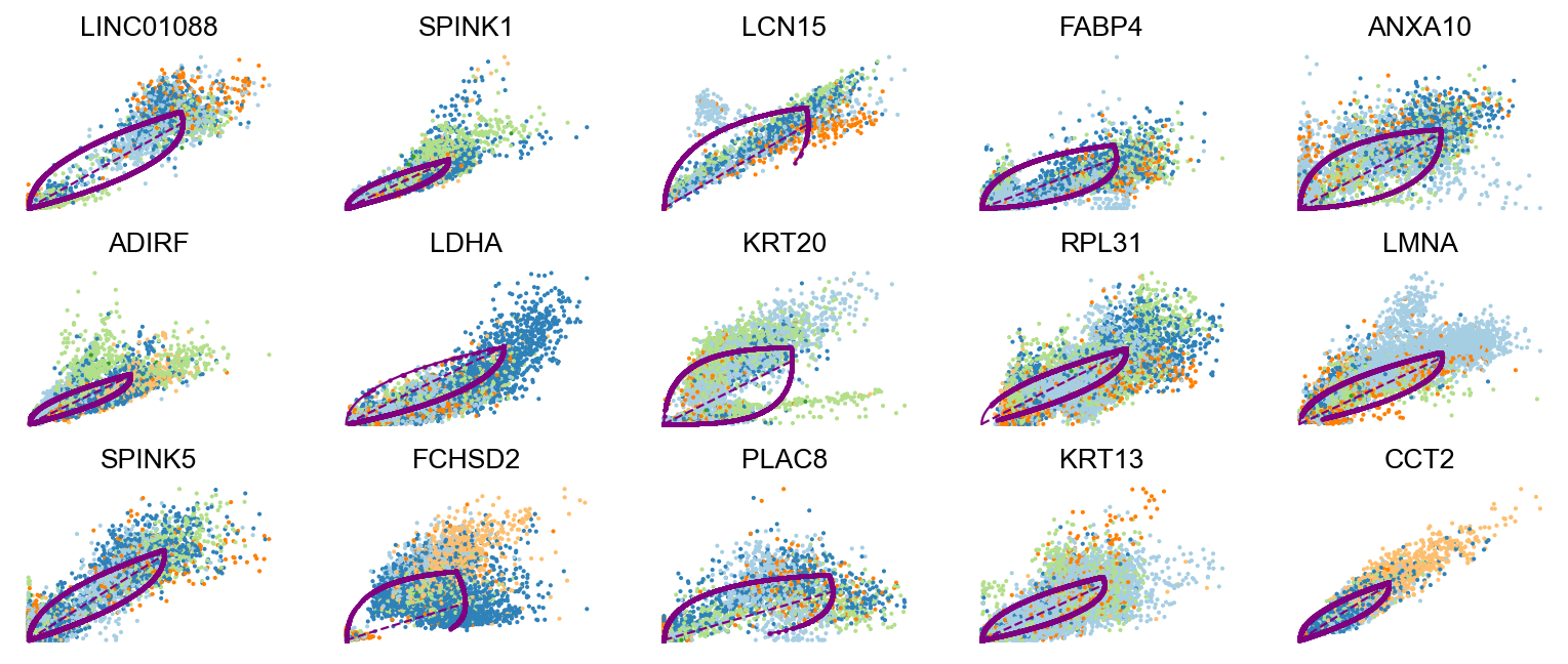
Driver genes display pronounced dynamic behavior and are systematically detected via their characterization by high likelihoods in the dynamic model.
top_genes = adata.var['fit_likelihood'].sort_values(ascending=False).index
scv.pl.scatter(adata, basis=top_genes[:15], ncols=5, frameon=False)
var_names = ['EMP1', 'FABP4', 'LDHA', 'FOSL1']
scv.pl.scatter(adata, var_names, frameon=False)
scv.pl.scatter(adata, x='latent_time', y=var_names, frameon=False)Moreover, partial gene likelihoods can be computed for a each cluster of cells to enable cluster-specific identification of potential drivers.
scv.tl.rank_dynamical_genes(adata, groupby='clusters')
df = scv.get_df(adata, 'rank_dynamical_genes/names')
df.head(5)
ranking genes by cluster-specific likelihoods
finished (0:00:03) --> added
'rank_dynamical_genes', sorted scores by group ids (adata.uns)
.dataframe tbody tr th {
    vertical-align: top;
}

.dataframe thead th {
    text-align: right;
}
| adhesion_signaling_luminal_cell | basal_cell | cancer_associated_luminal_cell | differentiated_luminal_cell | immunomodulatory_luminal_cell | unique_luminal_cell | |
|---|---|---|---|---|---|---|
| 0 | LCN15 | RPL31 | ANXA10 | KRT20 | ADIRF | FCHSD2 |
| 1 | FABP4 | ANXA1 | FCHSD2 | RPL31 | ZFAND2A | ANXA1 |
| 2 | LMNA | RAB11FIP1 | SPINK5 | TPM1 | SPINK1 | GPRC5A |
| 3 | MUC4 | GPRC5A | ADIRF | KRT13 | GPRC5A | ZFAND2A |
| 4 | LIMA1 | CLDN1 | UCA1 | TESC | GLA | CNOT2 |
kwargs = dict(frameon=False, size=10, linewidth=1.5)

scv.pl.scatter(adata, df['basal_cell'][:5], ylabel='basalCells', **kwargs)
scv.pl.scatter(adata, df['differentiated_luminal_cell'][:5], ylabel='diffLC', **kwargs)
scv.pl.scatter(adata, df['unique_luminal_cell'][:5], ylabel='uniqueLC', **kwargs)
scv.pl.scatter(adata, df['immunomodulatory_luminal_cell'][:5], ylabel='immuneLC', **kwargs)
scv.pl.scatter(adata, df['cancer_associated_luminal_cell'][:5], ylabel='cancerLC', **kwargs)-
EMP1 showed to be correlated with poor prognosis in bladder cancer ref
-
RPL31 is a ribosomal protein gene and can be omitted.
-
Both differentiated luminal cells and unique luminal cells shows simliar profiles. This can inidcate that these two clusters might be better to be merged as one cluster.
In datasets with multiple lineages and processes, genes may have different kinetics in various cell subpopulations. These differences result from distinct gene networks in different cell states, leading to multiple gene trajectories.
To tackle this, the dynamical model performs a likelihood-ratio test for different kinetics. This helps identify clusters with unique kinetics not explained by a single model. We can then fit each kinetic regime separately by grouping cell types accordingly.
Different cell types and lineages can have distinct kinetics due to variations in their gene networks. Even related cell types may show differential kinetics because of processes like alternative splicing, polyadenylation, and degradation modifications.
The dynamical model employs a likelihood ratio test for differential kinetics, identifying clusters or lineages with unique kinetics not well explained by a single model for overall dynamics. We assess each cell type's independent fit, checking if it significantly improves likelihood.
The likelihood ratio, which follows an asymptotic chi-squared distribution, is used to test for significance. Note that, for efficiency, an orthogonal regression is preferred over a full phase trajectory to evaluate whether a cluster has different kinetics from the overall pattern
# the following needs the dynamics to be recoverd before, if not it will take time to recover them

scv.tl.differential_kinetic_test(adata, groupby='clusters')
testing for differential kinetics
finished (0:01:28) --> added
'fit_diff_kinetics', clusters displaying differential kinetics (adata.var)
'fit_pvals_kinetics', p-values of differential kinetics (adata.var)
df=scv.get_df(adata, ['fit_diff_kinetics','fit_variance', 'fit_pval_kinetics'], precision=2)
df = df.dropna(subset=['fit_pval_kinetics'])
df.to_csv("diff_kinetics.csv")
df.dataframe tbody tr th {
vertical-align: top;
}
.dataframe thead th {
text-align: right;
}
| fit_diff_kinetics | fit_variance | fit_pval_kinetics | |
|---|---|---|---|
| Gene | |||
| RUNX3 | cancer_associated_luminal_cell | 1.85 | 7.58e-19 |
| MYCL | cancer_associated_luminal_cell,differentiated_... | 0.71 | 6.66e-08 |
| GBP1 | adhesion_signaling_luminal_cell,basal_cell | 1.30 | 7.36e-03 |
| ARHGAP29 | basal_cell | 1.66 | 3.78e-03 |
| AIM2 | basal_cell | 2.11 | 2.04e-04 |
| ... | ... | ... | ... |
| EGFL6 | basal_cell,cancer_associated_luminal_cell | 0.98 | 7.53e-04 |
| TSPYL2 | adhesion_signaling_luminal_cell,basal_cell | 1.69 | 2.02e-11 |
| MSN | adhesion_signaling_luminal_cell | 1.61 | 4.39e-06 |
| PRKY | adhesion_signaling_luminal_cell | 0.86 | 6.64e-105 |
| DDX3Y | basal_cell | 0.86 | 3.97e-03 |
217 rows × 3 columns
# Gene selection based on the fit_variance:
cancer_associated_luminal_cell = ['LCN15',]
differentiated_luminal_cell = ['SPINK1']
immunomodulatory_luminal_cell = ['LIPH','CCND1','CCT2','IRS2','RAB3IP']
unique_luminal_cell = ['ANXA1']
basal_cells = ['SHH', 'DSP','CXCL17','NRP2','TNNT3']


kwargs = dict(linewidth=2, add_linfit=True, frameon=False, figsize=(10,8))

scv.pl.scatter(adata, basis=immunomodulatory_luminal_cell, ylabel='immuneLC' ,**kwargs)
scv.pl.scatter(adata, basis=basal_cells, ylabel='basalCells' ,**kwargs)
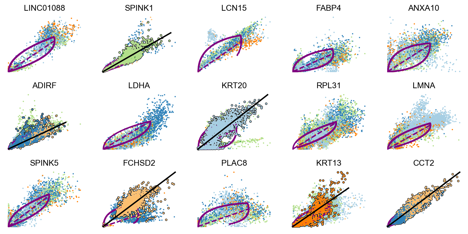
In the above plot for each genes, the kinetic behaviour is outlined, with the black line fitted through and the overall dynamics is showed purple curve.
# to get more genes
top_genes = adata.var['fit_likelihood'].sort_values(ascending=False).index[:100]
scv.tl.differential_kinetic_test(adata, var_names=top_genes, groupby='clusters')
testing for differential kinetics
finished (0:00:26) --> added
'fit_diff_kinetics', clusters displaying differential kinetics (adata.var)
'fit_pvals_kinetics', p-values of differential kinetics (adata.var)
scv.pl.scatter(adata, basis=top_genes[:15], ncols=5, add_outline='fit_diff_kinetics', **kwargs)scv.pl.scatter(adata, basis=top_genes[15:30], ncols=5, add_outline='fit_diff_kinetics', **kwargs)Finally, velocities can be recomputed leveraging the information of multiple competing kinetic regimes.
scv.tl.velocity(adata, diff_kinetics=True)
scv.tl.velocity_graph(adata)scv.pl.velocity_embedding_stream(adata, basis='umap', legend_loc='right margin', figsize=(10, 8), save= 'diff_kinetics_stream_plot.png')scv.pl.velocity_embedding(adata, basis='umap', legend_loc='right margin',arrow_length=8.0, figsize=(10, 8), save= 'diff_kinetics_embedding_plot.png')scv.tl.velocity_pseudotime(adata)
#scv.pl.scatter(adata, color='velocity_pseudotime', cmap='gnuplot')
scv.pl.scatter(adata, color=['velocity_pseudotime'], cmap='gnuplot')
