fth
this is not a direct port of the STUMPY Python library to an R package, instead showcases how-to setup Python modules in R with use of the reticulate library.
installation of stumpy using reticulate:
library(reticulate)

# py_install("stumpy", pip = TRUE)Time series motifs are approximately repeated subsequences found within a longer time series. Being able to say that a subsequence is “approximately repeated” requires that you be able to compare subsequences to each other. In the case of STUMPY, all subsequences within a time series can be compared by computing the pairwise z-normalized Euclidean distances and then storing only the index to its nearest neighbor. This nearest neighbor distance vector is referred to as the matrix profile and the index to each nearest neighbor within the time series is referred to as the matrix profile index. Luckily, the stump function takes in any time series (with floating point values) and computes the matrix profile along with the matrix profile indices and, in turn, one can immediately find time series motifs. Let’s look at an example:
This data was generated using fuzzy models applied to mimic a steam generator at the Abbott Power Plant in Champaign, IL. The data feature that we are interested in is the output steam flow telemetry that has units of kg/s and the data is “sampled” every three seconds with a total of 9,600 datapoints.
steam_df <- read.csv("https://zenodo.org/record/4273921/files/STUMPY_Basics_steamgen.csv?download=1")
steam_df |> head()
drum.pressure excess.oxygen water.level steam.flow
1 320.0824 2.50677390 0.0327013 9.302970
2 321.7110 2.54590790 0.2847994 9.662621
3 320.9133 2.36056150 0.2036516 10.990955
4 325.0025 0.02705418 0.3261869 12.430107
5 326.6528 0.28564943 0.7537763 13.681666
6 326.1869 2.63132810 1.8518541 14.608886
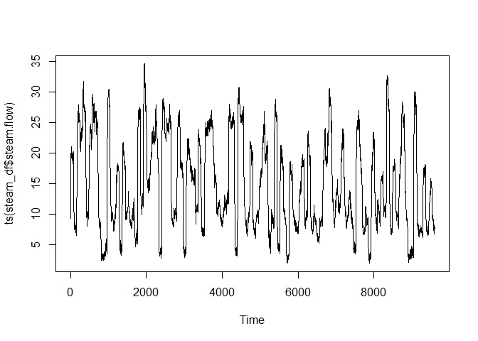
steam_df$steam.flow |> ts() |> plot()Take a moment and carefully examine the plot above with your naked eye. If you were told that there was a pattern that was approximately repeated, can you spot it? Even for a computer, this can be very challenging. Here’s what you should be looking for:
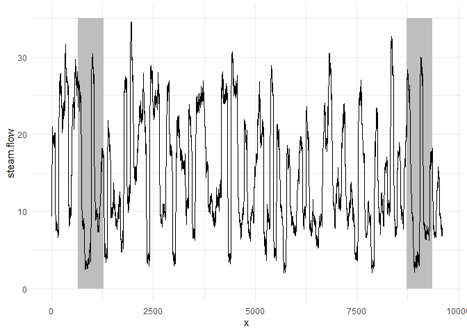
visualizing the motif again with dplyr + ggplot2:
library(ggplot2)
library(dplyr)
Attaching package: 'dplyr'
The following objects are masked from 'package:stats':
filter, lag
The following objects are masked from 'package:base':
intersect, setdiff, setequal, union
library(BobRossColors)

m <- 643

steam_df |>
  mutate(
    x = row_number()
  ) |>
  ggplot() +
  geom_rect(aes(xmin = 643,  xmax = 643  + m, ymin = 0, ymax = 35), fill = 'grey') +
  geom_rect(aes(xmin = 8724, xmax = 8724 + m, ymin = 0, ymax = 35), fill = 'grey') +
  geom_line(aes(x = x, y = steam.flow)) +
  theme_minimal()
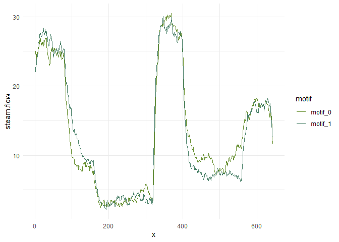
overlaying the sequences:
motif_0 <- seq(643,  length.out = m)
motif_1 <- seq(8724, length.out = m)

steam_df |>
  mutate(
    x = row_number()
  ) |>
  filter(x %in% c(motif_0, motif_1)) |>
  mutate(
    motif = c(rep("motif_0", m), rep("motif_1", m))
  ) |>
  group_by(motif) |>
  mutate(
    x = row_number()
  ) |>
  ggplot() +
  geom_line(aes(x = x, y = steam.flow, color = motif)) +
  theme_minimal() +
  BobRossColors::scale_color_bob_ross(painting = "meadow_lake", type = "qualitative")
The motif (pattern) that we are looking for is highlighted above and yet it is still very hard to be certain that the orange and green subsequences are a match (upper panel), that is, until we zoom in on them and overlay the subsequences on top each other (lower panel). Now, we can clearly see that the motif is very similar! The fundamental value of computing the matrix profile is that it not only allows you to quickly find motifs but it also identifies the nearest neighbor for all subsequences within your time series. Note that we haven’t actually done anything special here to locate the motif except that we grab the locations from the original paper and plotted them. Now, let’s take our steamgen data and apply the stump function to it:
import python library into R environment
stumpyr <- reticulate::import("stumpy")access the underlying STUMPY submodules with use of the dollar sign,
$
this takes place of the . in python examples.
$ is typical base R behavior, one can extract a column from a df with the same method (seen below):
# my experience with other python/r ports,
# params need to be set to int, R defaults to float/numeric,
# use as.integer() to set type

m  <- as.integer(640)

mp <- stumpyr$stump(steam_df$steam.flow, m)
stump requires two parameters:
-
A time series
-
A window size, m
In this case, based on some domain expertise, we’ve chosen m = 640, which is roughly equivalent to half-hour windows. And, again, the output of stump is an array that contains all of the matrix profile values (i.e., z-normalized Euclidean distance to your nearest neighbor) and matrix profile indices in the first and second columns, respectively (we’ll ignore the third and fourth columns for now). To identify the index location of the motif we’ll need to find the index location where the matrix profile, mp[:, 0], has the smallest value:
# mp |> ts() |> plot()
# mp |> as.data.frame()
# mp |> as.data.frame() |> str() # interesting, each value is a list object

# motif_idx = np.argsort(mp[, 0])[0]
motif_idx <- mp[, 1] |> unlist() |> order() |> head(1)

paste0("The motif is located at index ", motif_idx)
[1] "The motif is located at index 644"
With this motif_idx information, we can also identify the location of its nearest neighbor by cross-referencing the matrix profile indices
nearest_neighbor_idx <- mp[motif_idx, 2] |> unlist()

paste0("The nearest neighbor is located at index ", nearest_neighbor_idx)
[1] "The nearest neighbor is located at index 8724"
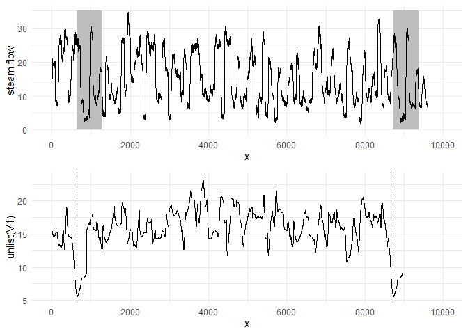
Now, let’s put all of this together and plot the matrix profile next to our raw data:
gridExtra::grid.arrange(
steam_df |>
  mutate(
    x = row_number()
  ) |>
  ggplot() +
  geom_rect(aes(xmin = motif_idx,
                xmax = 643  + motif_idx,
                ymin = 0, ymax = 35), fill = 'grey') +
  geom_rect(aes(xmin = nearest_neighbor_idx,
                xmax = 643  + nearest_neighbor_idx,
                ymin = 0, ymax = 35), fill = 'grey') +
  geom_line(aes(x = x, y = steam.flow)) +
  scale_x_continuous(breaks = seq(from = 0, to = 10000, by = 2000), limits = c(0,10000)) +
  theme_minimal(),

mp |>
  as.data.frame() |>
  mutate(x = row_number()) |>
  ggplot() +
  geom_line(aes(x = x, y = unlist(V1))) +
  geom_vline(aes(xintercept = motif_idx), linetype = 2) +
  geom_vline(aes(xintercept = nearest_neighbor_idx), linetype = 2) +
  scale_x_continuous(breaks = seq(from = 0, to = 10000, by = 2000), limits = c(0,10000)) +
  theme_minimal()
)
What we learn is that the global minima (vertical dashed lines) from the matrix profile correspond to the locations of the two subsequences that make up the motif pair! And the exact z-normalized Euclidean distance between these two subsequences is:
mp[motif_idx, 1] |> unlist()[1] 5.49162
So, this distance isn’t zero since we saw that the two subsequences aren’t an identical match but, relative to the rest of the matrix profile (i.e., compared to either the mean or median matrix profile values), we can understand that this motif is a significantly good match.
Conversely, the index location within our matrix profile that has the largest value (computed from stump above) is:
# discord_idx = np.argsort(mp[:, 0])[-1]

discord_idx <- mp[, 1] |> unlist() |> order() |> tail(1)

paste0("The discord is located at index ", discord_idx)
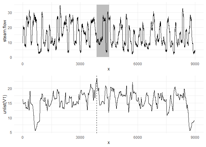
[1] "The discord is located at index 3865"
And the nearest neighbor to this discord has a distance that is quite far away:
nearest_neighbor_distance = mp[discord_idx, 1] |> unlist()

paste0("The nearest neighbor subsequence to this discord is ", nearest_neighbor_distance, " units away")
[1] "The nearest neighbor subsequence to this discord is 23.476168367302 units away"
The subsequence located at this global maximum is also referred to as a discord, novelty, or “potential anomaly”:
gridExtra::grid.arrange(
steam_df |>
  mutate(
    x = row_number()
  ) |>
  ggplot() +
  geom_rect(aes(xmin = discord_idx,  xmax = 643  + discord_idx, ymin = 0, ymax = 35), fill = 'grey') +
  geom_line(aes(x = x, y = steam.flow)) +
  scale_x_continuous(breaks = seq(from = 0, to = 9000, by = 3000), limits = c(0,9000)) +
  theme_minimal(),

mp |>
  as.data.frame() |>
  mutate(x = row_number()) |>
  ggplot() +
  geom_line(aes(x = x, y = unlist(V1))) +
  geom_vline(aes(xintercept = discord_idx), linetype = 2) +
  scale_x_continuous(breaks = seq(from = 0, to = 9000, by = 3000), limits = c(0,9000)) +
  theme_minimal()
)
Warning: Removed 600 rows containing missing values (`geom_line()`).
